spreadsheetjournalism

Transparency, it’s wonderful – when it’s transparent. In fact, however, if that informational property is openly put in place but compromised at the same time by data that suffers from its own brand of opacity, then you have a problem – at least an analytical, if not political one.

Put more…transparently, it means that if the information so freely disclosed isn’t technically sound, the view gets dimmed, all the good-government intentions notwithstanding.

Case in point: the UK parliamentary expense data recounted by the Guardian  and sourced in the first instance on the Independent Parliamentary Standards Authority web site(click the Data Downloads link), and these workbooks in particular (some field names are defined and explained here):

AnnualisedExpenseData_12_13

expenses parliament 2013-14

UK taxpayers – a coterie which seems to include yours truly – will be happy to audit the trail of requisitions upon which their elected officials have tread, and a good deal of the evidence is here. The question that could be asked is about their quality.

Turning first to the AnnualisedExpenseData (British spelling, note) sheet, you won’t need me to duly note the gathering of MP (Member of Parliament) Names into one cell, and sorted by first name. One might be pleased to leave that reversal of the conventional data wisdom alone, but if in fact you insist on a by-the-book, second name sort ordering you’ll have to think about it. If you reach for the Text to Columns tool and plan on parsing the MP names by their space separator (see the   post) remember that you’ll need to clear out two blank columns here to the right of the original field, because text-to-columns data reassignments overwrite existing information in contiguous columns and you need two additional columns here because three MPs have three names each, a lovely complication that could be relieved by a rather enormous formula we haven’t the space to describe here. The realpolitik alternative, apart from relenting to the current names arrangement? Here’s one:

1. Insert a column between columns A and B. Call it Last Name.
2. Copy the contents of A to what is now column B.
3. Select the names in the B column (B2:B65) and conduct the following Find and Replace:

Find: *[space]

Replace: leave blank

That device should deposit a precipitate of last names only in B. The Find-Replace seeks out all initial text up to, and including, the first space (the asterisk signifyies a wild-card search term), and replaces these with absolutely nothing. The remainder – last names only. Now feel free to sort by column B.

Now launch a fast scan of all the monetary data. If your antennae are pitching and yawing you’ve tuned into the right frequency, because all the numbers have been aligned left, the hallmark gauge of a text format. But we’re in luck. If you enter

=COUNT(D2:D658)

In cell D659 and copy the expression across all the number-bearing columns (ignore the results’ current format) you’ll get 657 every time, authenticating the numeric status of all these entries. Whew. You may still want to realign all these expense figures right, though, after which you could start to think about what one could make of them (an absence of MP party affiliations impairs the analytical prospects here, to be sure).

The second sheet – expense parliament 2013-14 – should prove more forthcoming, as it specifies, categorizes, and dates each expense item, thus conducing toward some interesting aggregations. You could, for example, splash out this pivot table:

Row Labels: Expense Type

Values: Amount Claimed (try sum and/or average, formatted to two decimals and with commas, or the 1000 separator, as Excel insists on calling it)

Amount Claimed (count)

(The below shot excerpts the whole.)

(You may note by the way that the Status column declares 10576 of the 10580 expense requests were paid in full).

In any case, once you’ve autofit the columns you could delete the Year column, containing as it does the undifferentiated 13_14 indication. But apart from another instance of first -name-first rendering of MP names another, familiar spectre haunts the data as well, one before which of which I need to issue a mea culpa of sorts. You may recall that my August 15 post on the massive UK food-inspection data decried the apparent fact that all dates featuring a day number greater than 12 presented themselves as text. I was somehow, and largely, wrong about that, in large measure because my grizzled laptop was set to the American date protocol, even as the data are expressed in European month-first syntax.

If you enter

=COUNT(B2:B10581)

in cell B10582, assuming it’s your B column that’s storing the date data, you’ll return 5132. Remember that COUNT only ticks cells containing numeric data, and as such it appears as if half the cells in B are something other than numeric – namely, text. Yet if you make way for a new column, say between B and C, call it Month and enter in C2

=MONTH(B2)

and copy it all the way down, you’ll discover that the month is realized for each and every B entry – as if each and every one of these were duly quantified, and not all of them really are, as our previous COUNT demonstrated. Moreover, the dates can’t be grouped, befitting data at least some of whose records are text-stamped.

I can’t authoritatively explain this inconsistency – namely why half the dates in B are reckoned as text (the Number Format field in the Number button group call them General, imputing them clear textual characteristics), and yet yield actual months when subject to the above unction. Suggestions, anyone? (See also my March 7 post for an account of a similar issue.)

But in any case, because the numbers do seem to work, more or less, you can easily push through a pivot table such as this one:

Row Labels: Month

Values: Amount Claimed (sum, formatted to two decimal points and a comma):

Hmmm. So anarchic is the monthly variation in expense claims that my primeval uncertainty about the date data churns anew – particularly after essaying this pivot table:

Row Labels: Month

Values: Month (count)

Half the expense claims were apparently filed in April, the month in which the British tax year culminates. In addition, if you substitute DAY for MONTH in the C column (and rename the field correspondingly) and run this table through the machinery:

Row Labels: Day

Values: Day (count)

You’ll see

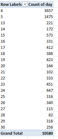
That is, a massive lopsiding toward the 4^th and 5^th days of the month – and absolutely no expenses claimed on the 31^st of any month, besides.

Are these overwhelming monthly and daily skews some quaint British quirk of parliamentary scheduling? I doubt it, but let me ask my wife – she’s British. Be that as it may, maybe we have some kind of story here, or maybe we have nothing at all. In the meantime, I’m on holiday next week– but I need to think about all this. Move to adjourn.

Please indulge your correspondent in a bit of analytical back-track, kinda sorta.  Last week’s post on the New York Police’s stop-and-frisk data, circa 2011, called our collective attention to the data curiosities in their midst, e.g, 8-foot, 999-pound suspects plunging their size 52s into the city’s sidewalks; and apart from one unstoppable question, namely, how these superhumans could be made to fit into a squad car, I guessed that these outsized numbers denoted data entry errors or lacunae, and as such I moved to detach all the records estimating suspects’ weights at 400 pounds or more.

Now that maneuver makes perfect sense, provided that you’ve nominated suspect weight your variable of analytical choice. But at the same time, it’s most likely that the height/weight exaggerations pollute the entries of actual stops-and-frisks; and as such you’d probably do well to readmit these dodgy records into the data fold by deleting the interposing row I fitted in last week – unless again, you’re interested in sizing up suspect weights. But on the other hand, the lapses uncovered to date (along with any blank cells in there, and there are) may augur still others; in other words, remain vigilant.

In any case and once you’ve seen to it that the time parameters I described in part 1 are duly columned, you can move on to consider your pivot table options, comprising nothing if not a dense buzz of possibilities. The most obvious, in view of the putative racial skewing of stops-and-frisks, is the tabling of race itself, simply executed:

Row Labels: Race

Values: Race (by Count)

Race again (by % of Row)

(again, it’s perfectly legal to impose the same field twice upon the same pivot table. The field is in effect breaking itself out).

Sieving the blanks via the Row Label filter button (and you know you’re dealing with a large set of data when 22,000 blank records amount to merely 3% of the whole), I get

Of course, you’ve already taken note of a problem here – the fact that race is numerically, not textually, coded. However, the New York Civil Liberty Union’s informative codebook deciphers the numbers:

1-Black

2-Black Hispanic

3-White Hispanic

4-White

5-Asian/Pacific Islander

6-American Indian/Native Alaskan

(While we’re at it, New York’s five boroughs receive these codes:

1-Manhattan

2-Brooklyn

3-Bronx

4-Queens

5-Staten Island )

The disparities are thus perfectly clear here, although these naturally await interpretation (see, for example this account. Note as well that the spotlight was trained on the stop-and-frisk issue during much of New York mayoral primary campaign, the votes for which were conducted two days ago).

But another potentially instructive breakout, namely stops-and-frisks by police precinct, suffers from some shortfall in quality control. Precinct numbers are keyed to their respective boroughs here:

http://www.nyc.gov/html/nypd/html/home/precincts.shtml

But run this pivot table:

Row Labels: Borough

Pct

Values: Pct (count)

And you’ll find a number of misassociations – though again, these contribute but an infinitesimal proportion of the whole – about 80 in toto. You’d have to wade through the data in order to correlate borough to precinct perfectly, though the fruits of that labor might not justify the exertions.

For another provocative read, try

Row Labels: arstmade (abbreviation for: was an arrest made? A code 0 represents no, a 1 yes)

Values: arstmade (count, % of column total):

We’re presented here with what are in effect nested proportions. African-Americans and Hispanics are a good deal more likely to be stopped and frisked, as we saw above, but once detained are less likely to be arrested than whites (code 4), – a metric that appears to comport with the racism thesis: that is, that police are relatively more likely to have less substantive cause to stop an African American or Hispanic citizen when they do.

If you then break the data out by age, say

Row Labels: Age (grouped in tranches of 5 years)

Values: Age (count)

You’ll find not shockingly that the 15-19, 20-24, and 25-29 cohorts account for about 63% of all stops and frisks, though taxpayers will want to know why the police also pulled over 13 320-to-324 year-olds. Data check, please.

And if it’s seasonality you want, try tabling the data by month, e.g.

Row Labels: Month (remember we introduced this field to the data)

Values: Month (count)

Month again (count, % of Column Total)

We see March was the busiest month, August the idlest, and I’m not sure why; the differential of over two absolute percentage points between the two is considerable and doubtless significant given the size of the data (with no blanks here, by the way; every record in the data set is dated).  After all, a 28-day February (remember, this is 2011) projects a chance-driven 7.67% of all stops; but it checks in at 8.88%, the third-most confrontational month. And the first six months of 2011 total 52.82% of all stops and frisks, the latter six 47.18%. Let the criminologists pause and reflect.

But given the welter of available fields, many more findings await. Just stop and frisk the data first.

Big data is a relative term, I’d allow. Redolent of prodigious, recondite servers and command-central cowboys programming their way through all that digital effluvia, big data could nevertheless be made to implode into spreadsheet dimension, comprising something like the 685,000 records overrunning the New York Police Department’s ledger of stop-and-frisk encounters for 2011. That workbook, a gorilla far too mammoth to be reposed in WordPress’s holding area, can be hauled up here:

http://www.tableausoftware.com/public/blog/2013/08/data-data-everywhere-2081

And you thought my 348,000 food ratings worth of data (August 14 and 21 posts) was big.

But once you’ve succeeded in finding a place in your creaking RAM for all those rows and columns – if you’ve succeeded – the analytical prospects massed within should justify the exertion. Stop-and-frisk searches of citizens who have, rightly or wrongly, been placed under on-the-fly suspicions of the potential for wrongdoing, are cause for perennial controversy in the States (see, for example this recent New Yorker piece), what with allegations that young African-American men are a good deal more likely to be placed under this sort of improvised scrutiny than everyone else; and so the data – which are, among other parameters, coded by race – are likely to beam some light on the matter.

But again, you need to get the workbook on your screen first. Truth to be told, I was surprised my proletarian, workaday laptop and its demotic 4-gigabyte  stash of RAM was up to the task, but it was, eventually, though you can probably wash your car during the time the file takes from call-up to appearance if your machine is similarly outfitted. When the smoke cleared following my first access, I found myself mano y mano with 232 MB worth of spreadsheet; but by liquidating columns that seemed unintelligible or less-than-serviceable, I managed to squeeze 129 MB worth of air out of the workbook – after which my RAM was able to exhale, at last.

And after which I was able to move from file to data management, where there was work to be done too. While many of the fields and their contents appeared self-evident and important, e.g., suspect height, ages, and weights – a few thousand or so weight readings seemed improbably, or impossibly large. Over 700 records featured suspect weights of 400 pounds of more, including a fearsome class of over 500 999-pounders – these, one assumes, data-entry proxies for no information. It’s hard to know where to draw the line here – there are 400-pound folks out there, after all – but there is where I drew it and introduced a blank row immediately before that number first appears, after having sorted by the weight field (it should be added that other parameters associated with these individuals – age, for example – seemed perfectly plausible). By the same token, it’s hard to know what to make of the detainees listed at 36 inches tall; it’s not inconceivable these were children, but some pause need be given here and at the other end of the ruler as well, at which 90-plus inch suspects have likewise apparently been sighted. And I remain clueless about the 20 one-year-olds who seem to have been subjected to police scrutiny.

Those issues matter, to be sure, but two other fields call for a more thoroughgoing think-through. Datestop and timestop, respectively, denoting the date and time at which a putative suspect was stopped, both exhibit the barest, unqualified numerical form e.g.:

(Pct, by the way, stands for police precinct.) That first date stop means to report December 7, 2011 (remember these are US-formatted data); its associated time purports to evaluate to 19:24. But that date is, in its present incarnation, nothing but 12,072,011, and its time merely 1,924. Any intention to group or otherwise understand the data in the spirit in which they were clearly intended needs to be anticipated by a tweak or two.

Turning to the dates, we can entitle ourselves to a breezy disregard of each record’s final four digits, because the spreadsheet devotes itself to 2011 data – and a result those digits teach us nothing we didn’t already know. It seems to me the simplest expedient here is to isolate month and day outcomes in independent columns, rather than jump through some formulaic ring of fire culminating in a wholly transfigured, actual date. I’d inset a column, then, between B and C, call it Month, and enter in C2:

=VALUE(IF(LEN(B2)=8,LEFT(B2,2),LEFT(B2,1)))

This expression looks at the number in B2, inquiring after its length – which should comprise either 7 or 8 digits, either/or because the data don’t sport trailing month zeros. If the length is 8, the formula simply captures two month-signifying digits from the value’s left; otherwise, it dusts off but one. Couching the expression in VALUE prepares the result for numerical grouping, in the event you want to so treat the data (the implication clued here then is that, absent the application of VALUE, the results will assume textual form).

Then add a column between what is now C and E, dub it Day, and enter in D2:

=VALUE(LEFT(RIGHT(B2,6),2))

 That careening between LEFT and RIGHT seems a little dizzying, but it works like this: We can infer, through an inspection of a sample of values, that, in contradistinction to months, every day does present two digits, including a trailing zero when necessary. Since we know that the six rightmost digits in every entry contain day and year information, we can carry away the two leftmost digits of those six, and that’s what the formula endeavors to do, that is: take the six rightmost digits from each cell value and from these uncouple the leftmost two. Again, VALUE quantifies the result.

The Time variable jams a stickier wicket into the turf, though, because of time’s 24-hour, 60-minute nomenclature. A stop-and-frisk-recorded time of 2055, for example, is simply not re-readable as 20:55, and the variable lengths of the time expressions here – two to four characters – throws another pylon into the road (54 in the data, for example, presumably means 00:54, and 140, 1:40). To make some usable sense of the data, I’d set these suggestions forth:

Clear out a column between E and G, head it Hour, and in F2 write

=VALUE(IF(LEN(E2)=2,0,IF(LEN(E2)=3,LEFT(E2,1),LEFT(E2,2))))

Welcome to a nested IF statement, and note the syntax therein, which declares the following: if the time reading in E2 amounts to three characters, then return a 0 in the formula cell, because again, a two-digit number must register a time in the midnight (00) hour. If, on the other hand, the cell offers three characters, grab its first digit (denoting hours 1 through 9). If neither condition is satisfied, that is if in effect the cell comprises four characters, then pinch two characters from the cell’s left. Note that the last-cited condition appears solo, not joined to an IF; that’s because it serves as a default, fall-back consequence when no other condition is met.

And if you need minute data, force another column, this one between what is presently F and G, call is Minute, and enter in G1:

=RIGHT(F2,2)

 That’s all. We can afford the simplicity here because all the time data cells seem always to devote their right two characters to minute data (understanding, of course, that some cells consist of only two characters).

One last point for now – I told you it’s a big file; don’t try to save it too often, unless you have another car to wash.