NHS Patient Waiting Times, Part 1: Weighting the Formulas

Divide finite resources by a spiking demand and the quotient shrinks, a mathematical truism all too pertinent to the UK’s National Health Service nowadays. Evidence of a system in crisis commands the country’s media and political attention, and of course data contribute integrally to the debate. One testimony – an NHS cataloguing of hospital treatment waiting times distributed by hospital and medical specialty – is here:

download-waiting-times-by-hospital-trust-xls-6289k-nov16-17215

The workbook’s front end comprises a Report tab, whose dropdown menus synopsize patient waiting time data for any user-selected hospital and treatment area. You may want to trace the contributory formulas, and note the lookups performed by the OFFSET function, about which we hope to say a bit more a bit later. Note as well the section topped by the Patients Waiting to Start Treatment reference data, vested in the IncompProv sheet; information about patients who completed their what the NHS terms their pathway and started treatment is displayed by the two recaps that follow, the first keyed to the AdmProv sheet, the second to NonAdmProv.

Those sheets – that is, the ones bearing the Prov term – are all comparably organized, each earmarking and cross-tabbing its first 19 records by medical speciality aggregates and waiting times, these expressed in one-week intervals. The next, 20th record then vertically sums the per-week totals; the remaining records break out the data by individual hospitals.

Those 20 aggregating rows loose a familiar complication upon the data sets, at for the pivot tablers among you. As per previous discussions, the rows in effect double-count the patient figures, by duplicating the hospital-by-hospital totals. And again, for the pivot-table minded, the weekly wait fields could have been more serviceably sown in a single field, for reasons which recalled numerous times.

But those impediments don’t daunt all efforts at analysis. You’ll observe the GT 00 to 18 Weeks SUM fields posted to the far reaches of the PROV sheets, these tabulating the numbers of patients obliged to wait up to 18 weeks for the respective attentions described in the sheets. I began to wonder, then, if an efficient formulaic way to measure patient waits for any number of weeks could be drawn up, and I came up with two (and there are others).

That is, I want to be able to learn for example how many General Surgery patients had to wait up to 14 weeks for treatment, by empowering the user to enter any medical specialty and week-wait duration (I’m assuming here that the wait is to be invariably measured from the inception of the wait – 0 weeks).

Assuming I’m looking at the IncompProv sheet – though what we do there should transpose pretty effortlessly to the other Prov data – I’d begin by instituting a dropdown menu of medical specialties, say in E1. I’d continue with another dropdown, this one unrolling the wait headers in set down row 3 (that is, the dropdown data – and not the menu itself – are to be found in row 3)..

I’d next select F3:B22, thereby spanning all the specialty aggregate names along with the week-wait values data. While the selection is in force I can muster an old but valuable option, Formulas > Create from Selection in the Defined Names button group. That run-through takes me here:

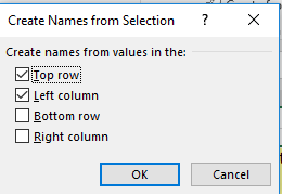
Click OK and each row and column in the selection receives a range name coined by the label to its left or immediately above its column (note that labels themselves are not enrolled in the range, and Excel’s reference to values in the above may mislead you. The ranges here are all textual). And by way of a final, preparatory touch, I’d consecutively number the weeks right above their columns in row 2, assigning 1 to 0-1 Weeks, 2 to 1-2 Weeks, and so on.

Remember we’re attempting to tally the aggregate number of patients awaiting treatment in a selected speciality for from 0 to a specified number of weeks. Per that agenda, I’ll enter the number of weeks – that is, the maximum specified week wait – in F2. Let’s say I enter 15, and then proceed to click on Ophthamology cell F8. I’m thus instructing the budding formula to calculate the number of patients who awaited treatment in that speciality for a period of up to 15 weeks. Next I’ll enter the formula, say in E2:

=SUM(OFFSET(INDIRECT(CELL(“address”)),0,0,1,F2+1))

I sense an explanation is in order, so here goes. In the final analysis, of course, the above expression sums patient numbers for the given specialty across a variable number of weeks – in the example, 15; and the formulaic potential to confront those variables is realized here by the OFFSET function.

OFFSET offers itself in two syntactical varieties, one requiring three arguments, the other five. The lengthier version, applied here, serves to identify the coordinates of a range, which will in turn submit itself to the SUM. In our case, the first of OFFSET’s arguments gives itself over to the INDIRECT function, itself performing a cell-evaluational role upon the nested CELL(“address”) expression. CELL(“address”) will, upon a refresh of the spreadsheet (triggered by the F9 key or some data entry elsewhere on the worksheet), return the address of the cell in which the cellpointer currently finds itself. Thus, for example, if you enter =CELL(“address”) in A12 and proceed to enter a value in C32, the function back in A12 will return $C$32 – the cell reference, not the cell’s value. But $C$32 is a textual outcome, i.e., not =$C$32. INDIRECT then restores a bona fide cell-referring status to $C$32, and reports the value currently stored in that cell.

So what does this have to do with our task? This: click on any medical specialty in F3:F22 and refresh the sheet. The address of that specialty populates OFFSET. For example, click on the name Ophthalmology refresh, and OFFSET will turn up F8, for our purposes the first cell in the range we’re striving to define. The two zeroes that follow tell OFFSET to in fact to define the range precisely at the F8 inaugural point – that is, not to move any rows or any columns away from that F8 range anchor. The 1 next instructs the formula that the imminent range comprises but one row – the row on which the Ophthalmology data are resting; and the F2+1 measures the range’s width in number of columns – in our case 16, or 15 plus 1 – plus 1, because the data for week 15 stand in the 16th column from the medical speciality in which we clicked to initiate the formula.

The answer in this particular case, then, is 330,472, counting of the number of ophthalmology patients who had to wait up to 15 weeks to receive treatment; and you could divide that figure by the Ophthalmology patient total – VLOOKUP(CELL(“contents”),F4:BH22,55,FALSE) – to learn that about 86% of the patients were waiting up to 15 weeks for treatment. So again, by clicking on Ophthalmology in F8 and refreshing the spreadsheet, the formula is put to work.

But there are other formulas that will work, too.