Archive | November, 2017

Burlington, Vermont Property Sales: Buying into the Data

24 Nov

House hunting? Then why not think about setting up stakes in Burlington, Vermont? Bucolic but sophisticated, a university town festooned with postcard-perfect New England autumnal foliage, lovely this time of year… and the very city in which Ben and Jerry’s Ice Cream was founded.

What more could you want? But the real reason I’m so keen on Burlington – a city I’ve never actually visited, after all – is its spreadsheet-archived history of property transactions, a veritably sociological, 100-plus-year account of the residential flux of its citizenry, available to you on Burlington’s open data site, and here, too:

Burlington Property Sales

All of which begs a first question about those 100-plus years: how complete is the sheet? Once you’ve done the column auto-fit thing, if you sort the data A to Z by column G – Sale_Date, whose holdings presently appear before us in text mode, you’ll observe that the three transactions in the data set lifted to the top of the sort are dated January 1, 1800, and succeeded by another seven sales, each of which was apparently conducted on July 14, 1897. Add the exactly twelve property purchases agreed upon in the 50s and the 21 more ratified in the following decade, and the market is starting to look a little sluggish, isn’t it?

I’m no developer, but I’m a speculator; and I’m speculating that the sales record as we have it must be partial, for whatever reason. I’m also conjecturing that the Sales Prices (column H) amounting to $0 denote a property bestowal of sorts, perhaps from a charitable donor to a governmental entity. In fact, I put that $0 conjecture to the Burlington open data site, and await their reply.

And in light of those sporadic sale representations it might be sensible to confine our analytical looks to the records commencing with 1990, because purchases in the 70s number a none-too-profuse 41, and the sales count for the 80s – 137 – appears questionably scant as well; and so it seems to me that a first analytic go-round, at least, might sensibly push off at 1990, the inception of the decade in which the data uncork a quantum leap in activity. But needless to say, a reportorial consideration of the property sales would force a closer look into the pre-1990 lacunae.

That’s one issue. For another, inspect the Sale_Date entries in column G. As adverstised, each and every one of these appears to be textual, encumbered by the T00:00:00.000Z suffix that entraps the real, immanent dates in their cells. But a fix is available (really more than one is out there): select column G and apply this Find and Replace:

Burl1

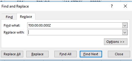
Replacing the suffix with nothing at all frees the actual, quantifiable dates within each cell, and even restores the results to my American regional date settings, in spite of their year-first formats.

But you may notice nine recalcitrants to the above workaround – the sale dates preceding 1900. They’ve shed their T00:00:00.000Z appendages but remain steadfastly textual; and that’s because Excel can’t directly process, or quantify, dates falling before January 1, 1900 (for some suggestions for allaying the problem look here). In light of the discussion above, however, that sticking point won’t adhere here, because our intention is to ignore sales predating 1990 anyway. But at the same time leaving those insistent textual entries in the data set will effectively stymie any attempt to group the dates in a pivot table; throw even one text datum into a date mix and you just can’t group it, or at least I can’t. Thus if you click on any date in the Sale_Date field and sort Oldest to Newest, the nine textual charlatans drop to the bottom of the column, whereupon one can thread a blank row immediately above them, and break them off from the remainder of the data set.

The larger question – albeit an academic one here – is to ask about a strategy for contending with say, a few thousand pre-1900 dates among the data, had they been there.  With a number that large, we would want to use them – but then what? The simplest tack, I think: not to run the Find and Replace, then, but rather draw up a new field in the next-available N column, call it something like Year, and enter in N2:

=VALUE(LEFT(G2,4))

and copy down N.

The reason we’d look past the Find and Replace here is because the above formula will return the pre-1900 postings as simple numbers, e.g. 1800; and 1800 doesn’t represent the year 1800. It stands in fact for December 4 1904, the 1800th day of the sequence commencing with the date baseline January 1, 1900 (and we’ll ignore Excel’s February 29, 1900 willful error taken up in the article linked above). In the interests of consistency, we’d want to regard the all the data in G one way or the other: either as bona fide dates or unvarnished numbers – and if we found ourselves working with pre-1900 dates we’d have to resort to the latter plan.

But again, because in our case the pre-1900 data are so negligible we’re ignoring them, and reverting to the actual date-making Find and Replace scheme. All of which at last enables the answer to an obvious research question:  how many Burlington properties have been purchased by year?

Start with this pivot table:

Rows: Sale_Date

Values: Sale_Date (count, grouped by Years. Click the Filter button by Row Labels, tick Date Filters, and enter
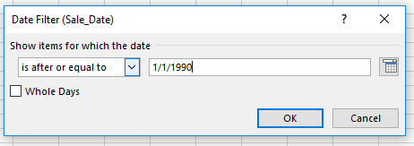
Burl2

I get:

Burl3

Note that the above Grand Total and its record complement date only from 1990, but nevertheless encompass 28790 of the 29032 entries packing the entire data set (note in addition that the 2017 data take the sales through September 15). The activity curve trends this way and that, with the numbers peaking in 2003 and scaling down erratically in the intervening 14 years (though all this of course assumes the data are complete for the respective years in hand, an unsubstantiated but not implausible guess).

We next might want to pursue a natural follow-up: an association of average purchase prices by year. But here too some forethought is needed – because by admitting the raft of $0 “purchases” into the calculations the averages would skew badly. We could thus apply a simple fix: take over the next free column (probably N; remember that the earlier data settlement in that column was hypothetical), call it Nonzero, and enter in N2:

=If(H2>0,H2,””)

H stores the Sales_Price data, and the “”, or length-less text double-quotes, will be ignored in any average computation. Once we expand the pivot table data source to N we can garnish the existing table with Nonzero, Average, and figured to two decimal points. I get:

Burl4

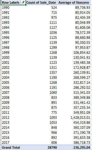
Unlike actual sales, the average prices proceed more or less upwards, an unsurprising ascent syncopated by the spike in 2012. Filter that year in the data set and you’ll find four identically described and dated purchases of $6,485,000, conducted on December 18 of that year by the Bobbin Mill Building Company and sold to the Burlington Housing Authority. A sweeping property acquisition by the powers that be, or a data-entry redundancy? I don’t know. And I haven’t come across any Land_Use and Deed_Type legends that would decode the entries in those fields, and that could inspire some additional breakouts of the data.

C’mon, Burlington, help me out here; give me those answers and there’s a Double Caramel Brownie Ben and Jerry’s cup in it for you. With an extra scoop – my treat.

World Series Winners and Losers: Playing the Percentages

13 Nov

Don’t be fooled by last week’s denouement of the World Series; the baseball season never really ends. The looks at the data from what was once boomed as the National Pastime just don’t stop, including some looks at the World Series itself, e.g. a survey put together by Joel Pozin of the regular-season winning percentages of Series participants dating back to the first series in 1903. It’s here:

Regular Season Winning Percentages of World Series Champions vs. Losers_ 1903-2017 Joel Pozin

The survey in fact contributes one of three small, public-domain Series’ datasets Pozin makes available on the collaboration-fostering data.world site (you’ll need to sign up for free for access to the other two workbooks; note that the percentage data for 1904 and 1994 aren’t there, because the World Series weren’t contested those years. In addition, I’ve appended percentage win-percentage data for the 2017 season to the sheet here.)

The other two workbooks recount the Series winner and loser percentages in their discrete sheets, but they do something else as well: they bare the formulas that return the team winning percentages, formulas that do a slightly different math from that performed by Major League Baseball’s number crunchers. A winning percentage, after all, emerges from a rather simple act of division: Wins/All games played. But Pozin has taken account of the mini class of games that, for whatever reason, culminated in a tie or draw, games that baseball officialdom simply bars from the win-loss calculation. Pozin, on the other hand, admits them to the All-games-played denominator, and assigns a .5 for each tie to the numerator. Pozin’s outcomes thus don’t invariably comport with the canonical percentages, though the differences of course aren’t game-changing, so to speak. But differences they are.

Those formulas themselves are interesting, however. On the loser sheet, for example, the 1903 Series runner-up Pittsburgh Pirates won 91 games, lost 49, and tied one, those respective accumulations committed to cells C2:E2 in the losers’ worksheet. The formula in F2 then declares:

=ROUND((C2+E2/2)/SUM(C2:E2),3)

(Note that the sheet featuring Series winners formulates its denominators this way instead, e.g.: (C2+D2+E2) ). The single tied game recorded in E2 is halved and added to the win figure in C2 to build the formula’s numerator; but in addition, the rounding of the result to three decimals quantifies the value in F2 to exactly what we see – .649, or .6490000.

But one could opine that the cause of exactitude could have been slightly better served with

=(C2+E2/2)/SUM(C2:E2)

followed by a formatting of the result to three decimals, thus preserving the quotient’s precision. The ROUND function forces a substantive pullback in precision – because after applying ROUND, the number you see is truly and only .649. But does my nit-pick here matter? Maybe.

And while we’re deliberating about things formatting, the winning percentages expressed in the workbooks in their Excel-default, 0.649 terms could be made to assume the baseball standard .649 deportment per this custom format:

series1

Now back to the winners and losers in the master sheet I’ve offered for download. A simple inaugural inquiry would have us calculate and compare the average winning percentage of the winners and losers. Rounded off to the usual three decimals I get .619 and .614 respectively, a dissimilitude that is neither great nor surprising. World Series competitors, after all, are the champions of their respective leagues, and so could be regarded as more-or-less equivalently skilled. And while of course only one team can win, the best-of-seven-game motif (in fact four series proceeded on a best-of-nine basis) could be ruled as too brief to define the truly superior squad.

But additional comparisons may point to other interesting disparities. If we pivot table and group the winning percentages in say, ten-year tranches:

Rows: Year

Values: ChampWinRatio (Average)

LoserWinRatio (Average)

(Remember that no Series was played in 1904 and 1994, and that the custom format we commended above must be reintroduced to the pivot table if you want it in play here. In addition, of course, the 2013-2022 tranche, forced by our grouping instruction to embody the ten-year amplitude, comprises only five years’ worth of data).

I get:

series2

Note the rather decided scale-down in winning percentages set in motion during the 1973-1982 tranche. Do these smallish but apparently real curtailments hint at a press toward parity among baseball’s teams that dulled the advantage of elite clubs? Perhaps the advent of free agency following the 1975 season, in which teams’ contractual hold on their players was relaxed, played its part in smoothing the distribution of talent.

But another, if distantly related, exposition of the trend could also be proposed. Baseball rolled out a post-regular-season playoff system in 1969, one that now qualifies ten of its 30 teams each season; and that broadened inclusiveness overwrites any guarantee that the clubs with the best regular-season records will find themselves in the fall classic.  The 1973 National League champion New York Mets, to call up the extreme example, beached up in the Series with a regular-season winning percentage of .509. But they won the playoff.

Now let’s return to my quibble about the deployment of the ROUND function, and my counter-suggestion for simply calculating win percentages without it and formatting the numbers to three decimals instead. Working with Joel Pozen’s rounded figures, we can write an array formula that’ll count the number of World Series victors whose regular-season percentage exceeded that of the losers each year:

{=SUM(IF(C2:C114>E2:E114,1))}

The formula assigns the value of 1 to each value in the C column – the one containing Series winners’ percentages – that tops the corresponding value in E, the losers’ column, and then adds all the 1’s (note: the formula can surely be written in alternative ways). I get 57, meaning that according to Pozin’s percentages a jot more than half of all the 113 World Series wins went to the team with the higher regular-season percentage.  Again, not a shocker, but worth demonstrating.

Now if we array-calculate the number of Series winners with the lower of the regular-season winning percentages:

{=SUM(IF(C2:C114<E2:E114,1))}

I get 53 – but there are 113 Series for which to account here, and 57 plus 53 computes to 110.   It turns out then then that in three Series – the ones played in 1949, 1958, and 2013 – the competing teams appear to have achieved the same regular-season win percentage.

And for two seasons, 1949 and 2013, the winner-loser identity is inarguable – the teams in those years had precisely the same numbers of wins and losses. But if we actuate my formulaic alternative, in which the drawn-game half-win-credit is retained but the ROUND function is shed for the reasons advanced above, we learn that the 1958 winner New York Yankees played to a .596774 percentage (rounded to six decimals), because they played a tie game that year; but the losing Milwaukee Braves steamed into the Series with a .597402. Seen that way, the 1958 Braves are the 54th losing team to best the winner’s regular-season mark.

The difference here of course is hair-splittingly slim. But if your head-of-the-class high school average was .000628 points greater than that of the runner-up, would you be willing to share your valedictorian honors by agreeing to a round-off?