spreadsheetjournalism

You can trace the course of justice in Chicago, including the direction and speed at which it travels, at the fledgling Cook County Government Open Data portal, a site brought to its URL at the behest of Kimberly Foxx, Illinois State’s Attorney for the county in which the city of the big shoulders shrugs. Four of the portal’s holdings –  Initiation, Dispositions, Sentencing, and Intake – chronologize the dispositions of cases processing through the system; I chose Sentencing for my look here.

It’s a big data set for a big city, recalling as it does sentencing records dating back to January 2010 and pulling through December 2017. With 189,000 cases and a field complement stretching to column AJ, don’t even think about calling it up in Google Sheets (the data-supporting capacity there: two million cells), but Excel is agreeable to its 41 megabytes if you are, and it’s available for download from the second above.

And at 41 megs, the minimalist in you will be avid to put your scissors to fields that might be rightly deemed dispensable. Cases in point: the four ID parameters fronting the data set in columns A through D, none of which are likely to advance your reportorial cause (note, by the way the interjection of commas into the large-sized identifiers, an unusual formatting fillip). Deleting the fields and their750,000 or so entries actually slimmed my workbook down to a lithe 29.7 mb, and that’s a good thing.

You may also note the slightly extraneous formatting besetting the INCIDENT_BEGIN_DATE, RECEIVED_DATE, and ARRAIGNMENT_DATE fields, their cells bearing time stamps all reading 0:00. I suspect these superfluities owe their unwanted appearances to the data in the ARREST_DATE field, which do exhibit meaningful times of suspect apprehension. We’ve seen this kind of excess before, but again it’s proper to wonder if any of it matters. If, after all, it’s your intention to re-present the data in pivot table form, for example, you’ll attend to any formatting disconnects there, and not here. If so, a reformatting of the data source may be no less superfluous.

But whatever you decide we can proceed to some analysis, acknowledging at the same time the scatter of blank cells dotting the records. Given the welter of substantive fields in there, quite a few possibilities beckon, and we could start by breaking out types of offenses by year, once you answer the prior question submitting itself, i.e. which of the available date parameters would be properly deployed here? I’d opt for ARREST_DATE, as it affords a kind of read on Chicago’s crime rate at the point of commission – or at least the rate of crimes culminating in arrest, surely a different and smaller-sized metric.

But if you’re thinking about installing the arrest dates into the column area, think twice – because the dates accompanied by their time-stamps are sufficiently granulated that they surpass Excel’s 16,384- column frontier. You’ll thus first have to swing these data into the Rows area, group them by Year, and only then can you back them into Columns, if that’s where you want them stationed.

And that’s what I did, only to be met up with a surprise. First, remember that Excel 2016 automatically decides upon a (collapsible) default date grouping by year, like it or not; and when I corralled the arrest dates into Rows I saw, in excerpt:

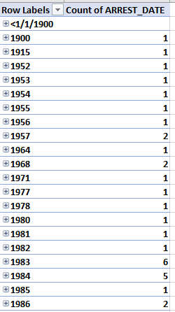
Now that ladder of years seems to be fitted with a column of rickety rungs. Remember that the sentence data appear to span the years 2010-2017, and so the aggregates above hint data entry typos, and at least some of them – e.g. the 1900 and 1915 citations – doubtless are.

The additional point, however, is that some of these putative discrepancies might tie themselves to crimes that were in fact brought to the attention of the justice system well in the past, and that took an extended while before they were actually adjudicated. Remember that our data set archives sentences, and some criminal dispositions take quite some time before a sentence is definitively pronounced.

For example, the 12 sentences associated with arrests made in 1991 reference serious crimes – seven murder or homicide charges, one armed robbery, one unlawful use of a weapon charge, one robbery and two thefts. One of the thefts, however, records an incident-began date (a separate field) of November 17, 2013, and thus appears to be erroneous.

But in any event, since our immediate concern is with arrests carried out in the 2010-17 interval I could click anywhere among the dates and proceed to group the data this way:

Note that I’ve modified the Starting at date to exclude the pre-2010 arrests, be they errantly captured or otherwise. Now after I click OK I can drag the years into the Columns area, after filtering out the residual <1/1/2010 or (blank) item.

Now I can drag OFFENSE_TITLE into Rows.

Surprise. With 1268 Offense categories cascading down the area you’ll have your work cut out for you, once you decide what to do next. Do you want to work with the data as they stand, or collapse near-identical types, and vet for misspellings along the way? Good questions – but in the interests of exposition we’ll leave them be.

How about something more immediately workable then, say age at incident? Exchange AGE_AT_INCIDENT for OFFENSE_TITLE, filter out the 2300 blanks, and group the ages by say, 3 years. Reprise AGE_AT_INCIDENT into Values (count). I get:

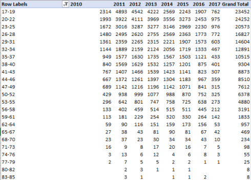
We see an extremely orderly negative association between age and arrests, with only the 20-22 tranche exceeding its predecessor bracket among the grand totals and only slightly. You’ll also observe that the numbers for 2017 are far smaller than the previous years, a likely function of incomplete data. In addition, track down to the Grand Totals row and behold the very significant ebbing of overall arrest totals from 2013 to 2016. Again, our table records arrest, and not crime totals, but the two likely point the same way – unless one wants to contend that the downturn in the former owes more to policing inefficiencies that any genuine diminution in crime – a not overwhelmingly probable development.

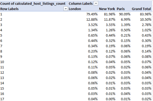
I’d then move to a Show Values As > % of Column Total look to learn how the brackets contribute differentially to arrests:

(The zeroes at the lowest reaches of the table reflect round-offs.)

Among other things, note the considerable, relative pull-back in arrests of suspects in the 17-19 range.

No, I don’t have an explanation at the ready for that, but perhaps you do.

There’s such a thing as overstaying your welcome, but Airbnb landlords – and in effect that’s what they sometimes appear to be – may be prepared to happily abide your long-term self, or selves, in their abode.

And that heartening show of hospitality may be illegal. They take a dim view of Airbnb’s good neighbor policy in London, for but one example, where the powers-that-be aren’t thrilled about the kind of lucrative serial subletting some Airbnbers perpetrate, straitening as it does the market for folks who’d prefer to hang tight in an actual, lease-driven apartment.

The long and the short of it then, is that it a review of Airbnb property availabilities – defined as the number of days in a year in which a given room remains on offer – could prove instructive, and our data for New York, London, and Paris devotes a field to just that question.

The analysis, then, should proceed pretty straightforwardly, once we do something about the startingly sizeable count of rooms – about 55,000 – that presently aren’t to be had. That is, their value in their dataset’s availability_365 field states 0, indicating that, for now at least, that room has been withheld from the market. An email from Inside Airbnb compiler Murray Cox informed me that zero means the property’s next 365 days in its calendar (presumably its start date is a moveable inception point, which Cox finds in the the scrape_date field in a different dataset) aren’t in play, at least temporarily.
And as such, those zeros – which are, after all, values that would contribute to and very much confound any formula result – have to be barred from the data set. Here I rely on my venerable highest-to-lowest sort of the availability_365 field, relegating the zeros to the bottom of the set; and once put in their place, an interpolated blank row immediately above the first zero will detach them from the usable data, for now (of course they can be recalled if needed via a simple deletion of the blank row).

And all that enables us to proceed here:

Rows: City

Values: availability_365 (Average, formatted to two decimals)

I get:

Real city variation is in force; and recall the linked article above, the one reporting the December 2016 London-approved bill “limiting Airbnb hosts to renting their property for only 90 days”. Looks as if a few thousand room owners in that city haven’t read the news lately.

We could next cross-tab the results by room type, by rolling room_type into Columns:

All the cities trend in the same direction, though not identically – itself a differentiation worth pursuing, perhaps. Availability widens as the rental space constricts, with shared rooms – defined by Airbnb as those in which “Guests sleep in a bedroom or a common area that could be shared with others”, presumably humans, who presumably might or might not be actually residents of the property – freed up for a considerably larger fraction of the year.

And the results make sense – even common sense, perhaps. Entire homes and apartments need be empty, by definition, and if so, where would their owners be expected to go for the duration of the rental?

That’s a good question, one that directs itself to one of flashpoints of the Airbnb controversy. Are its hosts the kinds of proprietors who hoard multiple listings that might otherwise be released to the conventional rental/purchase market?

A few sure-footed steps toward an answer would require us to divide all the rentals in a city by its number of hosts, i.e., an average of properties per host; and that simple division exercise needs to fill its denominator with a unique count of hosts, thus returning us to a problem with which we’ve tangled before. To reiterate it: an owner of multiple properties will naturally appear that many times in the data set, that is, once each for each holding, even as we want him/her here to appear once. In light of that complication I think the neatest way out this time is to conduct a Remove Duplicates maneuver (Data ribbon > Data Tools), and ticking the host_id field, the parameter whose entries contains the duplicates we want to shake out (again, you may want to save these results to a new workbook precisely because you’re shrinking the original data set).

But how do the host ids, once in their respective, solitudinous states facilitate a calculation of the number of properties they own, on average? Here’s how: once we’ve identified each host id singly, we can average the calculated_host_listings_count in column P via a city pivot table breakout. That field, which restates the number of each host’s holdings in each of his/her record entries, is one I would have deemed redundant to the data set’s design. After all, the owner-property count could otherwise be derived when needed, for example, via a pivot tabling of the hosts id, delivering the field to both the Rows and Values areas. But because we’ve removed all host id duplicates, that plotline has to be red-penciled – and that’s where the calculated_host_listings_count comes to salvage the script:

Rows: Country

Values: calculated_host_listing_count (Average, to two decimals)

I get:

We see then, that Airbnb hosts are for the most part single-property marketers, at least for the cities we’ve gathered. For those interested in more detail, we could try this:

Row Labels: calculated_host_listing_count

Columns: City

Values: calculated_host_listing_count (Count, % of Column Total, formatted in percentage terms to two decimals)

I get, in excerpt:

You get the idea, though we see London owners are notably more likely to offer multiple properties.

Speaking of which, croll to the bottom of the table above and you’ll find a 711, signifying the voluminous, apparent holdings of a fellow named Tom in London. But When I returned to our original, entire Airnbnb dataset, including the rooms for which availability was set at 0 days, I discovered but 350 properties strewn about London associated with his name.

Now Tom’s the kind of person Murray Cox wants us to know about; he owns so many properties that he’s lost track of half of them.