I wound up last week’s instalment with a measured augury about the promise all those 348,000 records held for the spreadsheet-minded, a fair appraisal to be sure, but one in need of an equally-sized codicil for ballast. Tuck a few hundred thousand lines of data beneath a slight, dull complement of fields, after all, and you’re not going to push the narrative terribly far. In fact, a plurality of fields probably trumps a towering stockpile of records, if you had to choose between those conditions, particularly if your analytical weapon of choice is the pivot table. More fields mean more permutations, and more possible, arresting takes on the data.
But back to the 348,000, and those dodgy takeaway/sandwich shop ratings diffused among them. In the interests of alternative accountings for those scores (some of which were put forward last week), it could be wondered if some skew in the inspection dates, rather than the doubtful sanitation of the eateries themselves, might be dogging the takeaway numbers.
And that interrogative takes us to the Rating Date field (you’ll want to autofit the workbook columns here, but you’ve probably made that move already), wherein you’ll be reintroduced to an old nemesis. It seems, again, that a great many of the dates here are formatted as text, a predicament that’s betokened by the intermittent left-right alignments marking the data:

To verify the surmise, streak down to the foot of the Rating Date column and enter:
=COUNT(D2:D384347)
(The above assumes of course that your dates inform the D column.)
COUNT, remember, only validates numeric entries in the range’s cells, and I get 132,421 of these. Put otherwise, about 215,000 of the rating dates are nothing but text, and as such remain resistant to the sorts of mathematical manipulations you’ll want to ply. I can’t explain this disparity, but there it is; and so in order to rehabilitate that contrary multitude here’s what I’d do, granting that alternative takes on the matter might be available.
Earmark the next three available columns Day, Month, and Year, and enter in J2:
=IF(ISTEXT(D2),VALUE(LEFT(D2,2)),DAY(D2))
To explain: You need an IF statement in order to customize respective solutions for cells bearing either text or numeric entries. The expression above asks if the item in E2 qualifies as text (that’s what IFTEXT does); if it is, then the formula chips off E2’s first two characters and runs them through VALUE, thus minting the result with quantitative standing. But if the condition isn’t met – that is, if the entry is already numeric (and remember that authentic dates are numbers) – then the expression returns the day of the month from the cell.
All of which raises two questions, one merely strategic, the other considerably more formidable. The first asks simply if you even want to bother with day-of-month data at all, as you may deem these too detailed for profitable scrutiny. The second points to the fact that none of those 130,000 genuine dates exhibit a number greater than 12 anywhere, bidding us to hesitate about their provenance. While it’s clear that the text-rendered data affect a European cast, e.g. 31/12/2012 (and of course the food ratings are British), that finding can’t be asserted with equivalent confidence about the 130,000.
In any event, assuming for the sake of exposition that all the dates, incipient or otherwise, have been habiltated in European garb, let’s move to the Month possibility, the data for which are centered in the date expressions. And indeed – because month data penetrate the interior of each record, neither the services of LEFT nor RIGHT can be required here (at least not directly). So I’ve written
=IF(ISTEXT(D2),VALUE(MID(D2,4,2)),MONTH(D2))
So what’s this one about? Again, we need to test the expression for its text status. If that be the case, we need to yank the month numbers from the heart of the entry via the MID function (see my September 13 post), then quantifying it with VALUE. (We can neatly specify 4 as a constant MID start number, by the way, because it appears as if all text-dates possess 10 characters, and so we know that the month identity announces its double-digited presence hard by the first front slash).
As for the Year field, try
=IF(ISTEXT(D2),VALUE(RIGHT(D2,4)),YEAR(D2))
And of course all these get copied down the respective columns.
Again, the permutations abound from here on, but you could start with a pivot table that goes something like this:
Row Labels: Year
Values: Business Type (Count)
Business Type (Count, Show Value as % of Column Total)
Rating Value (Average, formatted to two decimals)
Report Filter: start with Takeaway/sandwich shop
I get
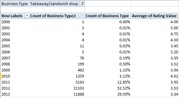
Hmmm. It’s still looking bad for the takeways, but nevertheless some association between recency of inspection and scores appears to obtain, particularly for the last two inspection years, when about 80% of the establishments were last reviewed. Try filtering for other business types, and you’ll note a systematic decrement in ratings starting with 2012 (though the School/college/university cohort seems to be holding the fort, more or less) – but however you slice it, you’ll find the takeaways consigned to a rear table.
On second thought, then, maybe I’ll eat at home tonight.

Leave a comment