Toiling with, and in, the Fields: Restructuring the Data, Part 2

If I may grab back the baton bearing the idea with which I had begun my sprint last week, you’ll recall I’d sung the praises of a certain manner of data organization, namely this:

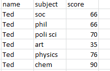
Rather than this:

(And yes, as Andrew Marratt commented last week, you can indeed do the work espoused here with Google/Open Refine (for a lucid tutorial on the data-righting process Refine calls transposing, see this post). Whether Refine does the deed identically, or more speedily or fluently is something one could talk about, but the option is in place. But for the sake of continuity we’ll honor the generic, delightfully retro Alt-D, P protocol. )

In any case, what ALT-D, P does among other things is trade in on the ambiguity between a field and a field item, by demoting the test subject fields with which we had started above to item status in a single, superordinate field, and you’ll recall as well that the routine’s dénouement comprised a double-click of the resulting pivot table’s Grand Total cell, which at last recombined the data into the recommended arrangement. And if you’re wondering about alternatives, guide our data through a standard pivot table (that is, sans ALT-D, P) and click Grand Total there; all you’ll do is replicate the data layout with which you started. And the larger is point looms: if here you want the pivot table to look like this

you’d be bidden to tug the subject fields into the Values area, and not Column Labels:

Because again, each subject continues holds to its field status; and if you do try and assign the subjects to Columns – something you might reflexively try –the subjects won’t line up alongside one another; rather, they’ll nest in precisely the superordinate-subordinate hierarchy that the Column/Row Labels areas always promote – and again, if that sounds impenetrably techie, try it, and you should see what I mean.  But pile all the subjects into the same field, and now your pivot table assumes your wished-for state:

And that’s what Alt-D, P does. It consolidates multiple data sets by strapping all the data into three generic Row, Column, and Values fields, perhaps in part because it has to be prepared to deal with variously-headed fields across the data sets.  Consolidate two data sets, each comprising three fields with incomparable names (and that’s something you can do here) and you’re left to pack them all into three consolidated fields – sporting six names. Three fields, six possible names – do the math. In the interests of decision-making, then, Excel fires three fields in the crucible, and names them, with all due practicality, Row, Column, and Values. Well, it beats Moe, Larry, and Curly.

But that’s all deep background, and if something’s been lost in the translation you can prevail nevertheless. The fact is that we’re not consolidating data sets here; we’re exploiting Alt-D, P for its three-column, data-digestible, revamping potential, and by way of another exercise we can return to the very scene of our original exposition – that very NPP file (which I’ve modified in the interests of pedagogical simplicity, by expurgating those fields that could be easily derived in a pivot table) about which I mused on September 28:

NPP_FPDB_PopulationbyGender take two

Remember that we want to single-columnize all those year/gender fields, the better to pivot table them (for all those reasons we’ve detailed above). Feed the data through the Alt-D, P process we stepped through in part 1, and you should be brought here (in excerpt below):

(My inclination here, and one you may not share, would be to entertain the TableTools > Convert to Range (in the Tools button group) possibility, so as to step over those nasty table-specific formulas – and you could also rename the field headings).

Now even as we’ve succeeded in reforming the data we’d almost surely want to break the Column data into the standard year and gender variables, a prospect that necessitates another, albeit more garden-variety chore. We need to in effect to split the Column data above into yearly and gender apportionments, and so I’d head the right-adjoining column Year and write, immediately below (assuming it all starts in row 1):

=LEFT(B2,4)

And copy down. As for the gender variable, I’d hop into the next column, call it gender, and write in E2:

=IF(RIGHT(B2,6)=”Female”,”W”,”M)

That is: if the cell’s 6 rightmost characters yield the term Female, register a W in the cell, and if the condition isn’t met, post an M therein. Copy down and you’re done. (You could also optionally impose a Copy > Paste Special > Values treatment upon these columns, and simply delete the Column column.)

Now you’ve granted yourself three substantive breakout variables – State (again, primevally called Row), Year, and Gender, for your pivot table delectation.