Location, location, location; and no, it’s not the real estate that’s got me waxing bromidic, it’s the spreadsheets, of course, and those recurring second thoughts about how their data are conveyed, and exactly how and where they’re…located.
Recurring, indeed, at least on these WordPressed pages; and apropos that perennial restiveness let us pack up and move to the Average House Prices Borough workbook on offer at the data.london.gov.uk site, and learn a little about that city’s combustible and ever-newsworthy real estate sector, and its no-less-combustible spreadsheet. It’s coming to your neighbourhood here:
The data here clamber about eleven scarily similar sheets, strewing price and sales volume numbers across the 33 London boroughs (they’re counting the interstitial City of London as a borough here). And while the data are readable, are they usable? That is, can you do something with them?
A loaded question, replete with half-full answers, because of course the answer depends. Take, for example, the identically-structured Median and Mean Annual sheets, asking after their receptivity to pivot tabling. My answer: iffy. The sheets, you will note, drape the data in year-per-field mode, e.g.:

And that peculiar positioning, as I took some pains to urge upon you in my August 22 and 29, 2013 posts, clogs the pivot tabling enterprise, and so if you want to effect the kind of data transposition I described there (but won’t belabor) here, you’ll need to:
- Delete the vacant row 2.
- Consider this: because the restructuring espoused in the August posts trisects the data into Row, Column, and Value fields only (which in turn are cast into a three-legged, or field, Excel Table), and because it is invariably the leftmost field in a data set that resets itself in Row terms, the Area field text data will assimilate into the Column field, even though its borough names are not of a piece with the numeric year data. What you could do, then, is simply delete the not-terribly-meaningful Code field, thus vesting Area – now the leftmost of the fields – with Row status.
- Earmark only A1:S34 for the pivot table-eligible makeover, that is, just the London borough-identifying rows. The summatory data beneath row 34 communicate different kind of data.
You could do much the same with the Mean Quarterly sheet, but their double-headed fields – Q1, Q2, etc. supervened by the year-referencing 2010, 2011, etc., in the merged cells in row 1, won’t work. Delete row 1 and rewrite the Quarterly heads to a differentiating Q12010, Q2010, and so on. (You’d need to do something similar with the Upper Quartile Quarterly, which for all the world sounds like a scholarly journal. Here, though, you’d have to pad the 1,2,3,4 quarterly headers with the year data instead.)
It’s also occurred to me that once you’ve submitted the data to the above process you could march on and develop pivot-table breakouts along Inner-Outer London lines, as per the aggregated Inner-Outer mentions in the lower reaches of most of the sheets and which won’t appear in the pivot tables we’ve commended above. (For a detailing of the Inner-Outer borough opposition see this piece. There is, by the way, a dispute about where the borough of Newham goes.) So once you’ve forced the data into the Row, Column, Value triumvirate you can then add a fourth field (say, called I/O, and that’s a not a computer throughput allusion) stocked with borough Inner-Outer identifiers.
To head in that direction you first need to hammer together a lookup table, the data for which I’ve carried off from this bit of real estate:
http://www.londoncouncils.gov.uk/londonfacts/londonlocalgovernment/londonboroughs.htm
|
Camden |
I |
| Greenwich | I |
| Hackney | I |
| Hammersmith and Fulham | I |
| Islington | I |
| Royal Borough of Kensington and Chelsea | I |
| Lambeth | I |
| Lewisham | I |
| Southwark | I |
| Tower Hamlets | I |
| Wandsworth | I |
| Westminster | I |
| City of London | I |
| Barking and Dagenham | O |
| Barnet | O |
| Bexley | O |
| Brent | O |
| Bromley | O |
| Croydon | O |
| Ealing | O |
| Enfield | O |
| Haringey | O |
| Harrow | O |
| Havering | O |
| Hillingdon | O |
| Hounslow | O |
| Kingston upon Thames | O |
| Merton | O |
| Newham | O |
| Redbridge | O |
| Richmond upon Thames | O |
| Sutton | O |
| Waltham Forest | O |
You’ll then need to edit the borough names here so that they correspond to those in the workbook, e.g., trim Royal Borough of Kensington and Chelsea, and keep an eye on Hammersmith and Fulham. Best practice: copy one instance of each of those two from the Row data into the lookup table.) Copy the table somewhere into the workbook, and call it say, InnerOuter. Then once you’ve put Row, Column, and Value in place, say with the Median Annual data, write this formula in D2 (after naming this new table column I/O):
=VLOOKUP([@Row],innerouter,2,FALSE)
Tables being tables, the formula automatically writes itself down the D column (the [@Row] syntactical bit is how Tables express a cell upon which you’ve clicked, instead of the standard A2, for example. They’re called structured references, and aren’t quite a day at the beach; see a Microsoft discussion here).
Once you fused the data thusly, e.g.:

(the formatting is basic Table defaulting at work)
You can pivot table this take, for one:
Row Labels: Column
Column Labels: I/O
Values: Value (Average, and formatted as you see here)
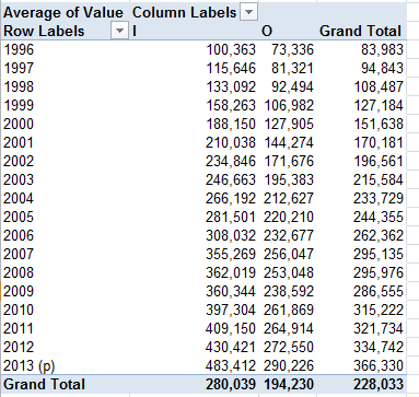
Remember those are median house prices cross-tabbed by year and Inner/Outer values.
I live in Outer London, by the way. Is that why Outer prices are so much lower?

Leave a comment