On this at least we can agree: that Donald Trump’s conversational style is not of a piece with say, that of Noel Coward or de la Rochefoucauld, not even the printable utterances. On the other hand, those latter epigrammarians were not able to run for the Presidency of the United States, and Mr. Trump is; and as he presses that Constitutional entitlement beyond what some might deem the breaking point it occurred to me the electorate might be productively served by a look at his Tweets, those on-the-record pronouncements issuing from the mind and the smart-phoning hand of the man who would be commander-in-chief (gulp).
And toward that end I returned to an old companion, the twdocs.com site and its Tweet-dredging apparatus, even as it now charges for its excavations. And so after shelling out $7.80 for the privilege, I was presented with a download of the candidate’s last 3106 tweets, those at least through February 11, two subsequent to his win in the New Hampshire primary. (I’m also not sure if I can present you in turn with my finished product for download, as I’ve paid for it. So until my legal department rules otherwise I suppose you’ll have to spend $7.80, too, understanding of course that, depending on the time and day on which you order your tweet collection, it’ll depart slightly from mine )
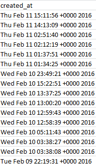
The first analytical order of business is to do something about the dates holding down the created_at field in the A column:

Surprise – they’re not dates yet, at least not by Excel’s formatting lights. All those +0000 2016s get in the way of proper date standing, as do the Wed, Tue etc. day-of-week qualifications that likewise can’t comport with the application’s date-reading defaults. But the task of repacking these now-textual data into usable dates is considerably trickier than I first thought, unless I’m missing something terribly elementary and decisive.
First break open a new column between A and B and call it Date. In what is now B4 enter:
=VALUE(MID(A4,5,15))
The MID puts the tweezer to the text label in A4, culling the 15 characters proceeding from position 5 in the cell. (We’re happy to take advantage of the fact that all the A-column data comprises 30 characters, freeing us to copy the above expression as it stands all the way down B.) And because that MID result remains textual, the VALUE supplement completes A4’s changeover to a duly accredited quantitative entry: 42410.56765. Reformat that handsome value to Short Date mode and the whole process culminates in an eminently usable 2/10/2016. So what’s tricky about that?
Not much, to be sure. The tricky bit doesn’t start playing up until cell B608, whose partner in the A column records the first of Trump’s 2015 tweets. B608 evaluates to 12/31/2016 – and that’s because considered alone, apart from some qualifying year reference, Dec 31 23:21:49 defaults to the current year (and it’s the two-year spread of the data here that works against approach to this problem I offered in this post). Enter 12/31 in any cell, after all, and Excel gives itself no choice but to assume that the implicit year in there is the self-same one in which the datum was entered. The 2015 in A608 won’t help, either, because the label Dec 31 2015 can’t be properly read by VALUE – but Dec 31, 2015 is automatically read as a date.
Thus if upon returning to B4 we try
=VALUE(MID(4,5,6)&”, “&RIGHT(A4,4)
That does seem to work.
That rewrite in effect string-concatenates “Dec 31, ” and “2015”, the latter having been made available through the RIGHT addendum, into Dec 31, 2015, and again Excel can re-evaluate that version into a bona fide date. (Note the “, ” interpolation, complete with the space that follows the comma.) You’ll observe, of course, that we’ve barred the time data from the expression, but we can still pull times out separately if we need them.
While you wait for the dust settles superimpose a Paste > Value from the B data back onto itself in B, and format the field in Short Date terms; now we can group the tweets by chronological units, as per this pivot table, for example:
Row Labels: Date (Group by Months and Years)
Values: Date (Count)
I get

The spreadsheet picks up on August 25, thus accounting for that month’s small accumulation, and again the February 2016 numbers halt at the 11th. The large October complement appears to feature many tweets Trump has quoted from other tweeters (these are apparently not categorical retweets), but even so doesn’t that possibility doesn’t explain the extent of quoting activity that month. Note that, even interpreted pro-rata, Trump’s February tweets fall behind January’s velocity, a slowing perhaps a creature of his stepped-up primary campaigning this month.
Now if tweet times-of-day do interest you push through a new column after Date, call it Time, and in what is now cell C4 enter
=VALUE(MID(A4,12,8)
That is, we’re reprising VALUE and MID here, this time recalling the eight time characters starting at position 12 in each cell. Again copy down the column, and Paste > Value atop itself. Then this pivot table should tell you want you want to know:
Row Labels: Time (Group by Hours only; turn off the default Months selection by simply clicking it).
Values: Time (Count)
I get

What I think is happening here – and I have to check with TWDocs on this – is that the tweet times have been transposed to my GMT zone, five hours ahead of the East Coast in the States. If I’m right, then the curiously high tweet total for 3AM really harks to 10PM Trump time.
But I’m not sure – let me tweet Mr. Trump and ask him.
Leave a comment