They say it only rains twice a week in Manchester – Sunday to Wednesday, and Thursday to Saturday. But I’ve been there, and after you’ve draped your socks over the radiator you’ll find it’s really not so bad. For one thing, the UK’s first free public library opened there (in 1653, when the United States was still an unlisted number in the Empire’s directory), and the first modern computer was fired up at Manchester University (in 1948, when Bill Gates was still an unlisted number in his empire’s directory). And I’ll bet you didn’t know its denizens are called Mancunians.
The city also has two contending, and contentious, soccer teams, but more to the point they’ve gotten with the open data program, too, in a small way for starters. Among their select data sets available to you and me is a record of license issuances to sundry food and clubbing establishments, more or less, an archive that should say something meaningful about the city’s commercial activities and direction; but perhaps more than the findings that await you’ll want to tilt your mouse at a number of spreadsheet challenges therein that you’ll probably need to confront if you want the data maximize their services on your behalf. In the interests of saving you a trip, you can get the workbook here:
Once you get past the need-to-autofit columns (as usual), and the analytically superfluous fields, e.g., EXTRACT DATE, ORGANISATIONURI, ORGANISATIONLABEL – all of which to appear to store the same information down their respective cells – you may want to turn to the LICENCESTARTDATE parameter and its longitudinal disclosures. And here you may encounter a problem – if you live in Manchester, New Hampshire, that is. The dates, after all, bear the imprint of their European-regional time format, whereby days of the month come first, and are only then followed by the month; and if your dates check cheque – out as dates, there’s nothing more for you to do.
But we contrarian Americans have it the other way around, of course, and if your pc shares that cultural idiosyncrasy the dates in our worksheet won’t behave very well at all. Those entries whose day of the month exceeds the number 12 simply won’t compute, and will thus be relegated to a fall-back status of text. To an American, 14/6/2012 reports a 14th month of the year, and our calendars don’t make room for that solar, or lunar, eventuality. Moreover, even while a date such as 6/3/2013 will cling to its native date format, American computers will insist on assigning the entry to the 3rd of June, and not the 6th of March on which the recorded event actually happened.
Of course you could reset your regional setting to a Euro-friendly one, but that overhaul is inconvenient and probably won’t play to sweetly to American colleagues; and if you try to simply replace the cells’ American cast with a rather standard Format Cells option, e.g.

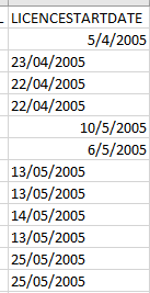
That exercise in the relatively obvious won’t work; or at least I couldn’t persuade it to cooperate, probably because the American regional setting hardwires its format so thoroughgoingly that the surface emendation above won’t root it out. The disparate cell alignments drawn from the workbook in the screen shot below capture the text/date duality:
Now we met up something similar in the very previous post on England National Health Service sick days, but there the ostensible dates, affecting this appearance:
2014-NOV
Seemed to be nothing but labels, each comprising the same character length, too, a prizeworthy asset for formula writers. But here in the Manchester workbook the lengths vary, owing to those single-digit days and months that aren’t paired with leading zeroes; and the length inconsistency will run roughshod over any formulaic attempt to work around it. That doesn’t mean that any such attempt will necessarily fail, because there are doubtless expressions out, or in, there that should indeed succeed in Americanizing all the dates. But their convolutions are…convoluted. Might an easier strategy be made to work?
Yes, in fact, and the strategy has been plotted by Alan Wyatt in his Excel Tips site, via a subjecting of the dates to a Text to Columns routine; we can get ours underway by selecting R2:R2266 and earmarking the backslashes as delimiters. Because the three columns to the immediate right of the LICENCESTARTDATE are conveniently and curiously empty, the first two of these will receive the newly-parsed month and year values into which the routine splits the entries, while LICENCESTARTDATE inherits the incipient day numbers (you may need to format the first of these columns into number mode, and decline its offer of two decimal points):

Once you’ve gotten here, settle into the abandoned OFFPREMISESALCOHOLSALE field, and enter in U2:
=DATE(T2,S2,R2)
Those references key themselves to the American month, day, and year protocol. Copy down U, copy-paste the values back to LICENCESTARTDATE and delete all the parsed data and formulas – and the European dates have been Yankee-imperialzed (after you’ve reformatted LICENCESTARTDATE into recognizable dates that is). You’ll also probably want to delete columns S and T; they’ve performed their roles admirably, and need not perform again.
Now you can begin to total licence approvals by year:
Row Labels: LICENCSESTARTDATE (Group by year. Note again that Excel 2016 will default to a year grouping.)
Values: LICENCSESTARTDATE (Count)
But if you’ve gotten this far you’ve already beheld, and surmounted, one of the challenges to which paragraph two here alerted you. The range to be pivot-tabled defaults somehow to AJ65536, even as the apparent data before us tops out at row 2266. Of course the value 65536 signposts the old row limit that boxed in Excel’s pre-2007 versions; and after caroming across the sheet I discovered approximately 63,000 putatively blank cells in the W column tracking back to row 2667, that bear five superfluous spaces each. I can’t account for these pseudo-nullities that inflict a real impact upon the sheet. Why these entries take us down to the old row limit, and why each and every one comprises five spaces stand as two good questions that should quite rightly be put to Manchester’s open data cadre. But they’re there, and should be deleted. And when you do, your year-by-year breakout of licence issues should read:

(Remember the above shot was snapped from the 2016 version).
The top-heavy 2005 count assigns us yet one more question, and I’m wondering if it happens to be clasped to the previous one. Perhaps some of those 63,000 space-bearing cells held licence records that, for whatever reason, were withdrawn from the workbook we have. I doubt that, but it’s a conjecture properly put to the folks in Manchester.
You may also want to train your investigative attentions on the LICENCEHOLDERPOSTCODE field, saying as it does something about the residential provenance and distribution of license holders (the spelling of license is as tricky as the inter-cultural date formats). Note that the field’s postal (some of us call them zip) codes are split into space-divided halves, the first half representing the more essential reference to the code’s locality. Thus, for example, British sportswriters often name-drop Wimbledon as SW19, bespeaking the tournament’s coded south-west London position.
If then you do want to reap the code first-halves only you could try something like this, say for the entry in X2 (M40 1UB):
=LEFT(X2,FIND(“ “,X2)-1)
Here we’re isolating the text to the left of the space, located by the nested Find minus 1, because we don’t want the space itself to figure in the result. But that formula fired a blank into my cell and many, many other cells down the column into which I copied it – because again, and again for whatever reason, those postal codes are preceded by a leading space – and that is the space FIND finds, not the one centered between the halves. And for good measure, many of the codes have no second half – they read something like M1, with no space at all.
I can’t explain these unwanted addenda and omissions either, but a workaround is (eventually) available. I think its neatest course goes something like this: in a blank column, say AD, enter
=TRIM(X2)
In AD2. TRIM, after all, squeezes the dilatory spaces from expressions, and once we’ve removed the air from our formulas we can try, say in the equally empty AE column:
=IF(ISERR(FIND(” “,AD2)),AD2,LEFT(AD2,FIND(” “,AD2)-1))
The IF(ISERR clause searches for those entries that return an error message when in fact there’s no space in there to be found; when it lands upon such a datum, it simply returns the now-trimmed datum in the respective AD cell.
Hey – no one ever said data don’t get messy. What do you say wes clear our heads with a walk in the rain?

Leave a comment