Welcome back to the next installment of spreadsheet cubism, in which the same data task is imaged from multiple formulaic vantages.
We’ve already submitted the NHS patient waiting data to two such looks, and here comes the third, an arrestingly different one; arresting, both because of its startling simplicity, and because its workings have been hidden in plain sight from Excel users for some time.
Again, our interest is in learning the number of patients waiting for an identified number of weeks for treatment in one of 19 different medical specialties (and we’re continuing to work with the IncompProv tab). Our vantage begins to come into view when we select the F3:BG22 range that rectangulates (it’s a word; I checked) the week-waiting numbers, bordered by medical specialty.
Then perform a pair of identical finds and replaces, first on F4:F22 and then on G3:BG3 – or the ranges that carry medical speciality and week-wait headers respectively:
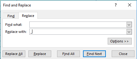
That is, replace every instance of a space among the earmarked cells with an underscore – yes, very much a to-be-explained step.
Re-select F3:B22 and turn next to an old Excel capability to which I’ve probably given rather short shrift, but have grown to appreciate of late – the Create Names from Selection feature, brought to you via the Defined Names button group in the Formula tab:

The default decisions above ascribe range names to every row and column in the selected range, the names coterminous with the labels in the range’s top row and left column – but you’ve probably figured that one out.
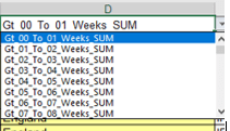
Our medical speciality dropdown-list menu remains in place in E1, and we’ll proceed to slot another dropdown in D1, this one comprising the week-wait labels in G3:BG3 (in fact the Treatment Functions Description in F3 likewise names its range, i.e. the medical speciality rubrics in F4:F22, but that name isn’t contributory to the process here). Then enter yet another dropdown in D2, referencing precisely the same range assigned to the menu in D1; and that apparent redundancy needs to be understood, of course (in fact you can simply copy D1 to D2; the menu will be duplicated).
And now, by the way – and this aside is far from incidental – we’ve learned why we needed to substitute the underscore for all those spaces a few paragraphs ago. Excel named ranges must comprise labels of contiguous text, and so when the spreadsheet meets up with a multi-worded header. it insists on exchanging a word-linking underscore for every space when it forges the range names. We thus had no choice but to do the same with the labels in F4:F22 and G3:B3, in order to anticipate and Excel’s range-naming mandate.
Now back to our budding formula. Say we want to learn the number of patients who have waited up to six weeks for treatment in oral surgery. Select that speciality in E1, and select Gt_00_To_01_Weeks_SUM in D1:
Tick Gt_05_To_06_Weeks_SUM in E2, because we’re counting patient numbers through week 6 for the oral surgery specialty.
Then, in a free cell, enter:
=SUM(INDIRECT(E1) (INDIRECT(D1):INDIRECT(D2)))
Which evaluates to 68,045, the number of oral surgery patients waiting up to six weeks for treatment.
That expression doubtless merits a to-be-explained as well. First, that is indeed a space insinuating itself between the first and second INDIRECT, and not a typo, begging in turn a rather pressing if rhetorical question: where does one find a space pushing its way inside an Excel formula?
You find it here. The space – and again, its functionality isn’t new to Excel – qualifies as an actual mathematical operator, of an operational piece with the traditional go-tos +, -, /, *. The space performs an act of identification: that is, in its base mode pinpoints a value standing at the intersection of two ranges. (And thanks to Jordan Goldmeier’s and Purnachandra Duggirala’s Dashboards for Excel, which promotes and explains the space operator approach.)
By way of a more straightforward introductory example, consider this assortment of test scores lined by student names and subjects, say in A1:G11:

(Note the collapsed space in the polisci entry, in anticipation of the Create from Selection’s name-underscoring practice.) Dubbing ranges again via the Create from Selection protocol, this unnervingly spare formula:
=Maureen[space]Art
returns 72, the value that stands at the confluence of ranges Maureen and Art.
The solution starkly pares the standard INDEX/MATCH solution to what is in effect this lookup task; indeed, so lean is the space-operator prescription that one is bidden to ask why it doesn’t predominate among users and commentators. I’m asking, but I don’t have the answer.
Now of course our denser formula departs from the above demo expression. For one thing it packs several instances of INDIRECT into the mix (see our discussion of that function here), because our three contributory dropdown-menu selections have returned merely textual references to the ranges with which we’re working, and these thus need to be synergized into actual, working range citations.
And the
(INDIRECT(D1):INDIRECT(D2))
half of the formula empowers it to find all the values dotting the intersections of the oral surgery specialty and all the columned ranges between and including the two we’ve actually identified in the formula; the space operator can do that, too (and note the placement of the parentheses, by the way).
And because the formula has sighted the multiple data points crossing their multiple intersections, the SUM function must gather these into a single total – our answer. Note that the standard INDEX/MATCH lookup can’t do carry out this additive step – at least I don’t think it can.
It’s probably worth your while, then, to learn more about the streamlining efficacy of the space operator. It’s been worth my while – and I’m lazier than you.

Leave a comment