spreadsheetjournalism

Thinking twice about cleaning the bedroom – you know, that bespoke chamber of horrors heaving in entropic fury, the one housing the bed on which you sleep – somewhere? If you are, then how many times would you think about cleaning New York playgrounds and parks?

How about 880,000, the number of tidy-ups the city’s Sanitation Department performed on its recreational spaces for the 2015-16 fiscal year? Mighty big number – but even so, they don’t do windows.

They do just about everything else, though, and a canvass of those 880,000 (more or less – please read on) contributions to New York’s civic betterment that have been carted into the data set on the city’s open data site may inspire you to consider haulage as a next-career move. (You’ll understand I’m much too nice a guy to force WordPress to absorb 130 MB worth of download from a greedy subscriber. You’ll need to get this one yourself, I’m afraid; just click the Download button on the above link, opting for CSV for Excel or CSV for Excel (Europe), the latter presumably flipping day-month entries in order to comport with regional defaults.)

But even if you put your CV on hold, the still data have something to say, though their fields call for a spell of reflection before you proceed, apart from the necessary auto-fitting of the several date fields. Indeed – your reflection may need to be rather sustained.

If, for example, you want to break out the task activity by New York’s five boroughs – and you probably will – you may want to extract the borough codes from the gispropnum entries in column A: B=Brooklyn, M=Manhattan, Q=Queens, R=Richmond (the official name for Staten Island), and X=Bronx (you may want to consult the helpful field descriptions here). It seems to me that convenience could be served by deleting the propid data in B (these code the city properties on which work was performed, but may not contribute substantively to your analysis, though you may decide otherwise), renaming the field Borough, and entering in B2

=LEFT(A2,1)

Copy the expression down B and the borough information readies itself for grouping, after which you could presumably run a Copy > Paste Values on the B results and delete A, again in the interests of economizing. You’ll also of course observe the Null entries, which presumably report on activities not carried out on site, e.g., Staff Pickup and Lunch.

You may opt for additional field deletions as well in light of the workbook’s size, and the corollary understanding that each such deletion will relieve the book of about 880,000 data-bearing cells. You may have little use for the vehicle_number information, for example, and perhaps route_id, though I suppose both dislodgings may have to be thought through.

But there are deeper concerns. One might want to begin simply, by pivot-tabling task totals by month of the fiscal year:

Rows: date_worked (grouped by months and years. Remember that this fiscal year was booted up on July 1, 2015)
Values: date_worked (% of Column total. You may want to turn off subtotals, and certainly Grand Totals, as the latter will ineluctably add to 100%).

I get:

Note the apparent, pronounced pullback of activity in September – though I don’t know why – and the orderly step-down in work from March through September, though of course that trajectory plots a seasonality course that runs backwards against the actual yearly grain.

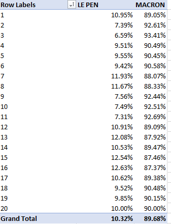
But that read isn’t necessarily that simple, or that accurate. That’s because a good many of the records seem to cite tasks that don’t quite qualify as an actual cleaning chore, e.g., lunch, De-Mobilization. So here’s a plan B: install the activity field in both the Columns and Values area, and in the latter, filter all activities save the one termed Work, which seems to serve as a catch-all item for…actual work on the parks. Continue to impose % of Column total on the values, and I get:

Once we’ve so trim the activity data – a retrenchment that abridges about 174,000 records from the whole – the monthly distribution redraws its curve. The conspicuous disparities bulge around July and August, each month here grabbing nearly two additional percentage points from the other months, even as the two September figures hold fast. Thus the obvious task-distributional suggestion – that non-work activity somehow features more numerously in July and August – remains obvious; but accountings for the numbers are not. I’m open to suggestions.

In any case, once we’ve put the work item in its place we could key the tasks to their boroughs, by exchanging the Borough field we fashioned earlier for date_worked. I get:

(Remember that N signifies the NULL entry.) It is perhaps notable that the assignments seem to have been similarly distributed across four of the city’s boroughs, with the far-less-populous Richmond well back. But these likenesses call for a deeper think, however, because they need to reconcile population (and of course Manhattan’s effective daytime census enormously exceeds its residential cohort) to aggregate park/playground counts and areas.
And what about the time expended on the tasks, again proceeding with the work-item filter as above? Here a New York open data field legend enters an important qualification about the nhours field: “A count of the adjusted number of hours a given task was performed [my emphasis].” You’ll see that for some instances – say row 43, a task whose start-to-end times evaluate to 35 minutes but is yet recorded by nhours as .292 hours, or 17.52 minutes – the lower estimate may reflect the simultaneous efforts of two workers, even as compensation of course would require the higher figure.
Going with nhours, then, we could replace activity in Values with nhours and format the resulting sums accordingly:

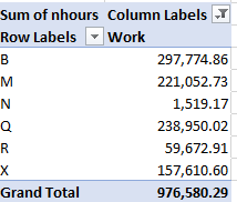
You’ll note that even as the task numbers stood as near-equivalents for Queens and the Bronx (the latter again represented by the letter X), work in the former borough seemed considerably more time-intensive.

Again, I don’t know why, but I’m just a spreadsheet guy, after all; if you want that Pulitzer you’ll have to take it from here.

Ok – you think you know who won the election, but in the interests of confirmation and deep background, you want to know how the French presidential runoff vote broke in Paris, don’t you?

Well, if you’ve made it this far, one supposes you do. The May 7 mano a mano – kind of – between Emmanuel Macron and Marine Le Pen culminated predictably in a flat-out triumph of the former, in both country and city, but even the obvious is properly reducible to its details.

You don’t need my pivot tables to learn that Macron won 89.68% of the determinate Paris vote (i.e., some other ballot casters voted but threw their support to no one via an empty form, and other ballots were voided), sustaining his hegemony in the city over his right-inclining opponent.  But for the deeper background (and again thanks to the folks at Open Data Paris) the data are here:

Election Results – Paris May 7

You can also download a far larger compendium of Paris election votes dating back to 2007 here.

Our workbook is identically organized, really an extension, of the document at which we looked in the previous post; but since of course the candidate count in our present iteration comes to two, the ensuing sheets look correspondingly sparer. Thus we can rerun this pivot table, after I named the prolix header in N “Candidate Vote”:

Rows: numero d’arrondissement 01 a 20

Columns: nom du candidat ou liste

Values: Candidate Vote (by % of Row Total; turn Grand Totals off).

I get, this time:

The table reports the overwhelming but irregular Paris mandate for Macron; considered in reverse, we see a comparative cresting of support for Le Pen in the well-heeled 16^th arrondissement and the adjoining but Left-Banked 15^th, and her bottoming out in the relatively hip, gentrifying 3^rd.

How do these outcomes square with the election’s first phase, run through on April 23^rd? Of course that competition distilled eleven candidacies into May 7^th’s two, and so a like-for-like retrospection need be conducted with some care. Still, we can play a useful trick on the April 23^rd data, by compiling an identically-conceived pivot to the one above, filtering the numbers for Macron and Le Pen alone. Thus slimmed, the table proceeds to regard the Macron-Le Pen vote as the operative whole, and computes its percentages accordingly.

That is, we can return to the previous (April 23) worksheet data, reconstruct the above table, and isolate Macron and Le Pen. I get:

Remember that Macron won 34.83% of the Paris April 23 vote overall, with Le Pen’s haul figuring to 4.99%; here their head-to-head relationship restores a couple of percentage points to Le Pen relative to the second vote; presumably her loss of ground in the finale speaks to the greater support thrown to Macron by the sectarians of the nine also-rans in the first go-round, and the decrement is fairly consistent across arrondissements. One glaring, provocative exception: Le Pen’s fall-back from 16.33% to 9.85% and a similar differential in the “ethnic” 19^th and 20^th respectively, these heavily Jewish and Muslim quarters. In light of those demographics, it’s the April 23^rd figures that give cause for surprise.

As for turnout, the analysis starts with a decision, or set of decisions, about definition. Does turnout emerge by simply dividing registered voters by all candidate votes, or do you toss in blank submissions (Nombre de blancs (uniquement) du bureau de vote), as well as ballots that, for whatever reason, were voided (Nombre de nuls (uniquement) du bureau de vote) along with proxy (presumably absentee, or Nombre de procurations du bureau de vote) ballots?

We broached this question in part in the previous post, but didn’t think the matter completely through. There we applied a formula that took into account the multiple counting of most of the parameters above, because each entry among the data recorded an individual candidate vote for a particular polling place, but at the same time repeatedly listed the number of blank votes, etc. – one listing for each of the eleven candidates on April 23.

In fact a simpler work-through appears to be available. On the May 7 sheet we can simply scoot to the bottom of the data set and enter a SUM function in cell N1794, thereby totalling all candidate votes. We can then enter SUMs in row 1794 for the other pertinent parameters and divide these results by 2, the number of times each polling place appears in the data set – that is, once for each remaining candidate (and yes, we could do the same for the April 23 data, dividing instead by eleven). But remember that the candidate-vote numbers in N are not subject to the divide-by-two restorative, because each record in N details a unique vote figure.

If then, we want quantify turnout via the number of candidate votes/number voters registered (nombre d’inscrits du bureau de vote, and yes; these are text entries that need to be converted back into values), we simply enter (somewhere) =N1794/H1794. That figure: 72.76%. The corresponding proportion for April 23: 82.71%, clearly, and notably, higher. The percentage of blank votes turned in this past Sunday: 4.44%, five times the .82% accumulated on the 23^rd. A statement was thereby made.

Now if we want to break out turnout by arrondissement – say here by dividing actual candidate votes by registrants by district, I named the arrondissement-bearing range in C2:C1793 arr, jumped into the free cell in S2 and entered 1, notched a 2 in S3, and filled down to S21, yielding numbers 1 through 20. In T2, then, I tried this formula:

=SUMIF(arr,S2,N$2:N$1793)/(SUMIF(arr,S2,H$2:H$1793)/2)

The expression sums all candidate votes (in N) by the 1^st arrondissement, per the entry in S2. It divides that total by all polling-place registrants in the 1^st, again dividing itself by 2 to offset the double-counting of each place (the votes in N don’t’ require that adjustment, because each record report a unique vote figure). After copying the formula down, I realized these turnout percentages:

In line with the April 23 data, the 19^th and 20^th exhibit lowest turnouts, even as we’ve operationalized them here.

For an index of sorts of disaffection, we can then calculate the blank-vote percentages, e.g.

=SUMIF(arr,S2,O$2:O$1793)/2/(SUMIF(arr,S2,H$2:H$1793)/2)

Note that here both numerator and denominator divide themselves by 2, because both elements need to fend off the double-count spectre (and note the placement of parentheses). I get:

Correlation between candidate vote turnout and blank vote proportions: -.54, pretty substantial and not shocking. After all, a preference for he, or she, bespeaks by definition a non-preference for no one.

So just to confirm, then: he won.