UK Immigration Raids: Migrating the Data

Designing a dataset falls on the complexity band somewhere between child’s play and rocket science, though I’m not sure to which of the poles the enterprise is closer. Rows and columns, you say; what else do you need, after all? And your rhetorical smirk is right, so far as it goes.

But sometimes the rows and columns require a think-through, preferably somewhere in that design stage – and particularly, for example, if the data are farmed out to more than a single sheet for starters.

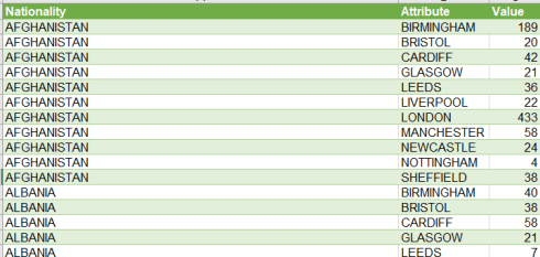
Case in point: the look, or pair of looks, at what the Bureau of Investigative Journalism calls Immigration encounters and arrests, a breakdown of city and nationality between January 2012 and January 2017 of individuals either questioned or arrested by law enforcement officials, presumably for a putative trespass of immigration law. The Bureau makes much of the large numbers of British citizens bunched with the foreign detainees, stoking the suggestion that these nationals, by definition entitled to be where they were when they were apprehended, were ethnically profiled, an inference the UK government discounts. The BIJ data are gathered here:

FOI 42354 – Annex A

(Observe the notes stationed beneath the data. If I understand the qualifications of note 2 on the ENCOUNTERED NOT ARRESTED sheet, the “total number of persons” seems to provide for the possible counting of the same person multiple times, should he/she be questioned more than once. Thus, the data appear to tabulate all encounters, not discrete individuals. And note 2 on ENCOUNTERED ARRESTED apparently makes analytical room for multiple arrests of the same person.)

And those data comprise two identically organized worksheets; and so, it seems to me, the pair should be pared. The likenesses among the two argue for a consolidation, but with a particular end in mind: to calculate the ratios marking the encountered and arrested figures, both by city of apprehension and origin of detainee (note: the misspelled city names Cardiff and Sheffield in the ENCOUNTERED ARRESTED sheet must be emended).

But before the consolidation comes the reconstitution. It’s something we’ve seen many times before, but because the worksheets assign field status to the several cities in the data set, these really need to be reined by the yoke of a single field; and to achieve that end we can review and apply Excel’s Power Query capability to the task, more particularly its doubtfully-named Unpivot feature.

First, and this script speaks to both data sets, delete the Grand Total column and row, the better to stem a double-count of the numbers. Then click anywhere in the data set and click Data > From Table/Range in the Get & Transform Data button group (remember I’m working in Excel 2016).

Next, select the fields to be incorporated into what Excel terms termed the attribute-value pairs (use the shift-arrow keyboard combination to select the fields) e.g. in excerpt:

Then click Transform > Unpivot Columns:

And follow with Home > Close & Load. The outcome should look like this, more or less:

But that doesn’t conclude the process, even when you’d do much the same as above for the second data set. We need to differentiate the records per their determination -that is, we need to clarify whether or not the stop culminated in an arrest. Thus we need to append a Status field to the results, coding and copying non-arrest outcomes Enc (Encounter, or something like it), and arrest dispositions, e.g. Arr, down the tables that require this or that status.

And once all that work has been carried out we need to merge the data, by simply copying one set immediately beneath the other – but that amalgamation stirs a small problem, too.

Note that when Power Query succeeds in unpivoting the data (and that verb won’t concede that the data it unpivots was never a pivot table to begin with), it refashions them into a table; and so when we perform the copy described above the copied table continues to retain its now-irrelevant header row, now threaded among the genuine records. But attempt a Delete> Table Rows of the header and Excel resists; the delete option is grayed out, because the second table – the one we’ve pasted beneath the first – remains a table very much in its own right, its positioning notwithstanding, and a table requires a header row, apparently. A workaround is at hand, though: click successively anywhere within the two tables and click Table Tools > Design > Convert to Range, and reply Yes to the prompt. Apart from gifting you with the answer to a question that has recurrently rustled your sleep – namely, when would you ever want to downgrade a table back to what Excel judgmentally calls a normal range – we’ve just learned the answer to a companion question – why? Here, converting a table, or tables, into ranges enables the user to delete the second, now superfluous header row, and agglomerate the two erstwhile, contiguous tables into a single unitary data set. And there are pivot tables in there for the gleaning. (And once these deeds have been done we could rename the default Attribute field City, and Value could be identified anew as Number.­)

And one such table, per our stated intention about 500 words ago, looks to discover the proportion of detainees actually arrested, broken out here by city:

Rows: City

Columns: Number

Values: Count (% of Row Total) Turn off Grand Totals.

I get:

We see, for reasons that remain to be expounded, some notable differentials. It appears that Bristol’s cohort of suspects – 1143 in absolute terms – was by far most likely to experience arrest, more than 120% more vulnerable to arraignment than Sheffield’s 4687.  But accountings for those disparities await, of course. It is at least possible, for example, to imagine that Bristol’s immigrant authorities proceeded with a greater precision, perhaps being guided by more trusted information. Far larger London exhibits a detention rate of 24.24%, a touch lower than the aggregate 25.30%.

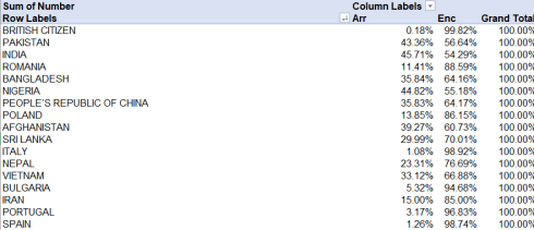
Substituting Nationality for City in the table and restoring Grand Totals yields a dossier of mixed findings, owing in part to the broad variation in the numbers of citizens for the respective countries. Sort by Grand Totals (the sort will work, even though they all display 100%; Excel sorts the values skulking behind the percentages), and the uppermost finding will give extended pause:

British citizens are practically never arrested when after being stopped for questioning, returning us to the proper question of profiling, and the kindred fact that the native British are stopped far more often – over 19,000 times that anyone else. On the other hand, we’re left to similarly explain Italy’s low arrest-to-encounter rate, or the fact the Norwegian nationals were stopped 32 times and never arrested.

Indeed, the mighty variation in rates begs a new round of questions; but the spreadsheet develops the first round of answers.