The decision to walk across the Brooklyn Bridge is a distinctly multivariate one, even if the internal equation that sets the walk in motion doesn’t chalk its terms on the walker’s psychic blackboard.
That preamble isn’t nearly as high-falutin’ as it sounds. Nearly all social activities negotiate trades-off between these and those alternatives, and a promenade over the bridge is no different. We’ve already observed the great, and expected, variation in bridge crossings by hour of the day in the previous post, and we could next consider the impact – if it’s proper to think about the matter in those causal terms – of month of the year on journey distribution (remember that our data records bridge crossings from October 1 2017 through July 31 of this year).
That objective calls for this straightforward pivot table:
Rows: hour_beginning (grouped by Year and Month. You need to put both of those grouping parameters in place in order to properly sequence the months, which straddle parts of two years.)
Values: Sum
Sum (again, here by % of Column Total)
I get:

The differentials are formidable, for me surprisingly so. One would have expected bridge foot traffic to crest in the summer, but a July-January walker ratio of 2.8 comes as a surprise, at least to me (remember again that the above totals compute one-way trips). It’s clear that meteorology has a lot to do with the decision to press ahead on the bridge, in addition to, or in conjunction with, chronology, i.e. the hour of day and day of the week. What we can’t know from the findings is whether the walkers had to get from Brooklyn to Manhattan or vice versa one way or another and chose to walk, or whether the trips were wholly discretionary.
And would one expect a spot of rain to discourage walkers? One suspects as much, of course, but confirmation or denial should be but a few clicks away. We could, for example, write a simple CORREL formula to associate precipitation with pedestrian turnout, provided we understand what it is we’re correlating. Here we need to remind ourselves that because we subjected in the previous post to a Get & Transform routine which replicated the pedestrian data source, that copy rolled twice as many rows we found in the orignal, assigning a record each to Towards Manhattan and Towards Brooklyn hourly totals. As a result each hourly precipitation figure is counted twice there, and so simplicity would have us look at rainfall data in the original dataset, if you still have it. If you do, this CORREL expression, which assesses precipitation by hour:
=CORREL(B2:B7297,H2:H7297)
Delivers a figure of -.0093, or a rather trifling fit between rain/snow and the determination to walk the bridge. Now that doesn’t look or sound right; but that perception is my way of saying it doesn’t comport with my commonsensical first guess.
But the correlation is “right”, in light of the manner in which I’ve framed the relationship. Because the formula considers precipitation with hourly pedestrian totals, most of the rainfall entries are overwhelmingly minute, and indeed, in over 4800 cases – almost two-thirds of all the hourly readings – amount to zero. The correlation appears to capitulate to what is, in effect, a host of unrelated walk/rainfall pairs.
But if you correlate walk numbers with aggregate rainfall by entire days the numbers read very differently. Continuing to the work with the original dataset, try this pivot table:
Rows: hour_beginning (grouped by Days)
Values: Pedestrians
Precipitation (both sum)
(Note that the row labels naturally nominate 1-Jan as the first entry, even as that date isn’t really the earliest. Remember the demonstration project got underway on October 1, 2017. But chronological order – really a lowest-to-highest numeric sort – is in no way a correlational necessity.)
Running a correlation on the above outcomes I get an association of -.333, which makes my common sense feel better about itself. That is, as calibrated here, rain “affects” pedestrian turnout to a fairly appreciable extent – the more rain, the fewer walkers, more or less. Again the (negative) correlation reflects the precipitation aggregated by days, not hours. Indeed – just 47 of the recorded 304 days report no precipitation at all.
And how does temperature figure in the decision to traverse the bridge? Again working with the original data set (and not the pivot table), in which each hourly instance appears once, we can rewrite the correlation, this time introducing the temperature field, which I have in the G column:
=CORREL(C2:C7297,G2:G7297)
I get .391, another persuasive, if partial relationship. With higher temperatures come stepped-up foot traffic – to a degree, pun intended – but that finding induces a couple of hesitations. For one thing, the Fahrenheit system to which the temperatures are here committed promotes an arbitrary, famous understanding, as it were – the temps aren’t keyed to an absolute zero. And so it occurred to me that a second correlation, this one redrawn with the temperatures pitched in Centigrade mode, crunch out a different result. That statistical hunch had me open a new temporary column (in my case in H), in which I refigured the temps with the cooperative CONVERT function, e.g.
=CONVERT(G2,”F”,”C”)
Copying down H and reprising the CORRELATION, this time with the C and H-columns range in tow, I wound up with… .391, at one with the first result, at least if you’re happy with a 3-decimal round-off, and I think I am.
But in fact the two .391s depart from one another by an infinitesimal sliver. The first, associating walk totals with temperatures expressed in Fahrenheit, comes to .390815536. That correlation with the temperatures in Centigrade (Celsius) calculates to .390959393. Presumably the tiny shift in numeric gravity wrought by the respective measurement systems accounts for the difference, about which few are likely to care, to be sure. But that discrepancy does mean I need to learn more about the workings of correlations.
The other caution about the correlation, whichever one chooses, asks about its linearity. While we could reasonably anticipate a swell in bridge crossings as the mercury ascends, it’s most possible, on the other hand, that pedestrian activity could be inhibited by temperatures forbiddingly high – in the 90s, for example.
And that conjecture could be submitted put to a pivot table (small note: two rows among the data record no temperatures), e g, assuming again we’ve remained with the original dataset, which features each temperature only once:
Rows: temperature (grouped, say, in bins of five degrees)
Values: Pedestrians (sum)
Pedestrians (count)
I get:
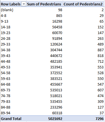
(The blanks reference the two empty temperature cells, and can be filtered out.)
The pedestrian count in effect totals the number of days populating each grouped temperature bin. After having filtered the blanks, move into the next-available D column – a space external to the pivot table – and enter in D4:
=B4/C4
Round to two decimal points and copy down D (I don’t think a calculated field can must this result). I get:

We’ve disclosed a strong if imperfect (and unsurprising) upward association between pedestrian hour averages and temperature. But the highest reading – 89-94 degrees – does seem to drive a pull-back in traffic. Note in addition the leap in hourly crossings from the 74-78 to 79-83 bins, as if 80 degrees or so lifts the inclination to walk to its tipping point.
So there. Didn’t I tell you the decision to lace up those high-heeled sneakers was multivariate?
P.S. In response to my previous post’s curiosity about a few missing Towards Brooklyn/Manhattan data, New York’s Department of Transportation wrote me that the empty entries might be attributable to a weather-induced snarl.

Leave a comment