Art and Gender at MoMA, Part 2: Drawing Some Conclusions

If there’s a Part 1 can a Part 2 be far behind? And while I’m answering the question only because you’ve asked it, the answer is yes.

There was a Part 1 to this distended duology of looks at gender at the Museum of Modern art compiled by Anna Jacobson, the party of the first part having been issued a president or so ago. Your patience is appreciated.

Part 1 counted the numbers of installations at MOMA dotting the 61 years between 1929 and 1989 plied by women artists, a sum greased by a couple of Excel’s new and cool dynamic array functions. OK; they’re not as new now as they were then, but that doesn’t mean they’ve overstepped their sell-by. Hardly; and in fact, curmudgeon that I am, I want to use them again. And the file, again:

Moma

How about, for example, a proportioning of gender by exhibition year – that is, an envisioning of exhibition numbers for each year along the male/female axis? Question 2: does that sound like a job for a pivot table? It sure does. After all, I want to see something like a column of years teamed with a perpendicular row of gender identifiers, and some numbers shipped into all those year-gender cell intersections – and that prospect has pivot table written all over it. But I want to apply the dynamic array strategy to the task for two reasons: one, to demonstrate exactly how it works, and two, to hint at a larger, looming intent, one possibly strategized by Microsoft: to position dynamic array functions as a formula-driven alternative to pivot tables, at least in part.

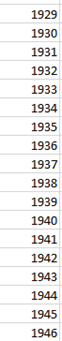
Let us begin, then, by minting a new sheet and raising that column of years, a step which in turn raises a question: because the date fields (e.g. ExhibitionBeginDate) contain precisely that – full-bodied dates – our formula needs to ferret just the years from those data, and pour these into the column. Given that necessity, this formula in say, C5, seems to work:

=UNIQUE(YEAR(ExhibitionBeginDate))

We’ve again mustered the dynamic array UNIQUE function (we called upon it in Part 1, if memory serves me correctly), which here braces the nested YEAR function that shakes out the years from the exhibition start dates i.e., in excerpt:

Now for the gender field and its peculiar requirements. We’ll return to the UNIQUE function in view of our interest in isolating a one-time instance of each discrete entry in the field. Move to D4 – one row up and one column to the right of B5, preparatory to roofing our matrix with its horizontal edge. Thus =UNIQUE(Gender) delivers:

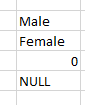
I didn’t say it would be pretty. We haven’t much use for the 8,700 empty Gender cells that have collected themselves up there with that 0; nor will we able to press ahead with the solitary entry for the Brazlian artist Roberto Marcelo, whose gender has somehow been reported as NULL. We want to offload these ciphers from our matrix-in-progress, and so we’ll submit the data to this close shave:  

=UNIQUE(FILTER(Gender,(Gender=”Male”)+(Gender=”female”)))

We’ve here recalled the dynamic array’s mighty FILTER function, introduced some time during last spring training, or thereabouts. In our case, FILTER is asking after records in the Gender field that exhibit either Male or (expressed by the plus sign) Female in its range, with the UNIQUE remaining in place.

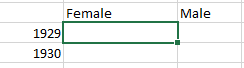
But if you’ve been following along you’ll understand that we’re not there yet, because our formula continues to return its output in default vertical orientation; and we want Male and Female to swing into horizontal place. We can make that happen thusly:

=TRANSPOSE(UNIQUE(FILTER(Gender,(Gender=”Male”)+(Gender=”female”))))

TRANSPOSE is an old Excel array function, greatly streamlined by the dynamic array regime. Befitting our task, TRANSPOSE flips a range 90 degrees either way – from vertical to horizontal or vice versa (and it works with multiple rows or columns, too). Next, clamp the dynamic array SORT around the expression – because, neat freaks that we are, we want Female to precede Male in its alphabetic scheme of things. Just make sure to get all those parentheses right:

=TRANSPOSE(SORT(UNIQUE(FILTER(Gender,(Gender=”Male”)+(Gender=”female”)))))

(Note that SORT follows TRANSPOSE in the above syntactical flow. Try =SORT(TRANPOSE( and Male will continue to precede Female. We see that TRANSPOSE does its work after all the other chores have been attended to.

Now all we need to do is fill all those blanks with the counts of female and male exhibitors by the years, and a count sounds like a job for COUNTIF – or COUNTIFS in this case, but in dynamic array style. That is, I want to develop a count of the number of female and male artists exhibiting at MOMA, and by year – with precisely one formula.

To start, drop into cell D5, the coordinate that sits to the immediate right and directly beneath the formulas that gave rise to the years and gender identities:

What we want, of course, is for COUNTIFS to cobble every permutation of gender count by year, naturally invoking year and gender criteria along with a third parameter – ExhibitionRole, which comprises six different identifiers (in addition to the pertinacious 0), only one of which is Artist.

First, while our matrix’s year column was able to scrape its years from the exhibition dates via =UNIQUE(Year(ExhibitionBeginDate)), it seems that COUNTIFS won’t honor that sort of second-order criterion. Rather, we’re bidden instead to nail a derived field of years to the next-available AB column in the source data sheet. Call it Years, and enter in AB2 the singular

=YEAR(ExhibitionBeginDate)

and nothing more. Again, the energetic dynamic array formula drives itself down AB, grabbing the year from each and every Exhibition Date.  Then post in D5 back in our matrix

=COUNTIFS(moma!AB2#,C5#,Gender,D4#,ExhibitionRole,”Artist”)

We’d entered something like this in the previous post, but not exactly like this. What’s different here, among other things, is the surfacing of those pound signs (i.e. hashmarks if you live in the UK), important indicators that require explaining. The sign attaches to a reference signaling the address of a dynamic array formula. Since, for example, our pillar of years springs from the dynamic formula we installed into C5, C5# identifies it as such, and here as a criterion in our COUNTIFS statement; and the moma!AB2# reference thus points to the dynamic array formula serving as a criterion range.

In any case, that COUNTIFS should make this happen (in excerpt):

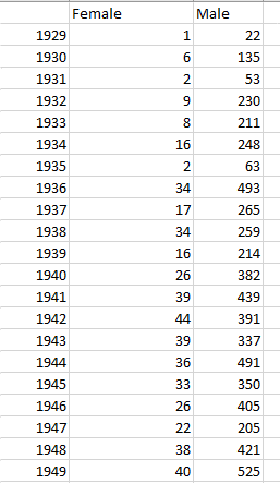
Indeed – note what’s happened, and why. We’ve fired a grand total of three formulas into the analytical fray and brought out 122 cells’ worth of results – two each for the 61 years separating 1929 from 1989; but had we been charged with tabulating 500 years’ worth of data we’d still be up to the task with just those three formulas. That’s what dynamic array formulas do. Note, for example, that the COUNTIFS picks up the numbers for both genders in both columns, thus casting its net horizontally and vertically.

And if you want to learn the yearly proportion of female exhibitors, one formula will do here, too. Try, in F5:

=D5:D65/(D5:D65+E5:E65)

The entire range of women contributors furnishes the numerator, draped atop a denominator of all the female and male artists. Get that done and you’ll find an appreciable, if fitful, uptick in women’s installations, though the 10.44% figure for 1989 is in actuality the smallest since 1980.

And if it at least looks like a pivot table, you’re right. Can Microsoft sue itself for plagiarism?