Last week’s cliff-hanger of a post pulled up at a familiar precipice, dangling its topical teaser from the edge of but one more data-formatting conundrum – a long skein of cells donning this – or that – format.
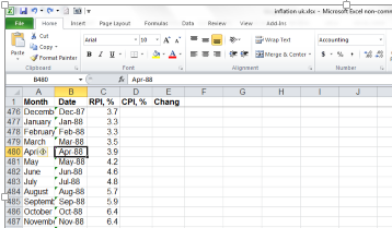
The cells in question skid down the B, or Dates, column in the inflation uk spreadsheet we introduced last week,s and they’re an eclectic bunch, styled in no fewer than three different formats, fitted out across four different ranges.
Cells B2:B488 – whose adjoining C column evince RPI data and whose adjoining vacant D and E columns have yet to receive any CPI and Change in weekly pay numbers – ostensibly dress themselves in the Accounting format, a standard numeric guise:
The problem is that the data bob and weave somewhere in the interstice between numbers and text. Click the Number Format drop-down arrow and textual evidence abounds:
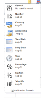
Authentically numeric data would appear in all their numeric finery beneath the Number rubric above, and under other headings, too. The Aug-81 you see, on the other hand, evidences something else – something decidedly non-numeric. Moreover, if you write:
=COUNT(B2:B488)
The function that counts cells in a range sporting numeric values, you’ll realize a grand total of 0. But if you multiply any cell between B2 and B488, e.g,
=B100*2
You’ll muster an actual, numeric result. Strange.
I can’t account for the bizarre duality visited upon these cells, other than to wonder if they’ve experienced some sort of mutation in the course of being spirited away from some other, primary source (that this format precisely blankets only those RPI data that precede the entry of the CPI figures at row 489 suggests an external provenance.)
In any case, a workaround is at hand. You’ve doubtless taken note of the green-notched alerts attaching to each and every cell in B2:B488; select the range and note in turn the exclamation-marked indicator and its clarifying legend:
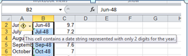
I will confess some uncertainty over the official standing of the “date string” phrase, but that’s my problem. In any event, clicking the exclamation mark uncorks two Convert options, and because all our dates are appear to be of 20th-century vintage, click Convert XX to 19XX (I don’t recall seeing these possibilities before either). Proceed and our problem range has been reformed into real, obedient, well-meaning dates.
You’ll be happy to know that the next 268 rows in column B are already irreproachably date-formatted, and that brings us to B757, at which the data seem to have been handed over, at least for the next 13 rows, to what the number format field in the Number button group reports as a Text format. There’s a quick fix here, too: click in I757 and enter
=DATEVALUE(B757)
DATEVALUE knocks some numerical sense into date-looking text, thus making them fit for all those pivot tables and formulas you have at the ready. Copy it down to I769, then copy those results, and apply a Paste Special to B757:B69 and take the rest of the morning off.
But the admirable efficacy of DATEVALUE got me to thinking: could we have done this same formulaic thing to B2:B489? It turns out we could have indeed; that is, we could have written
=DATEVALUE(B2) etc.
and emulate the very same text-to-bona-fide-numeric date rewrite that Convert XX worked out.
It seems the two text-laden ranges – B2:B489 and B757:B769 – share some genetic code, even though the former triggered the green notches and exclamation marks, and the latter didn’t. I can’t explain the disparity, other than to float the idea that these patches of data emanate from heterogeneous sources; your comments and conjectures are welcome.
And last and numerically least, cells B770:B777 revert to duly certified date format. Once you’ve unified the date format throughout the Date range and you can rev up the pivot tables and attendant date groupings, etc.
A few codicils: you’ll need to either delete the data-source attributing rows 778 and 779 or splay 777 and 778 with a blank row, thus exiling these extraneous text entries from the greater body of data. There’s also the matter of those month names gathering in the A column. I’m not sure what forthright advantage redounds to these unalloyed text data; we can already chisel months from the date data in B, after all. If for some reason you wanted to groups months qua months, absent their association with their respective years (e.g. the RPI averages for all Aprils), you could go ahead with the B-column data.
Of course the larger question is to ask why they data were compiled in the way in which they were, uncombed and contrary. I don’t know, and short of braving a query to the folks at the Guardian, the evidence suggests a polyglot workbook glued from shards of data prospected from hither and yon. The aim, again: get all the data to speak the same language. Esperanto, anyone?

Leave a comment