Face it: unless you’re an astrophysicist or a currency exchanger of epochal venality you’ve never had to add, subtract, or otherwise crunch a number that had to be cranked to 14 decimal points.
Until now. But it’s a data viz, map-happy, GIS-driven world out there, with latitude and longitude data dilating spreadsheet columns all across the net with DNA-sequence prolixity – and it’s your job to deal with them. Case in point: the directory of New York’s sidewalk cafés compiled here, and dredged from the New York City Open Data site:
There’s over a thousand spots served up here for your dining, sipping and passing-scene-watching pleasure, named, addressed, zip coded, and square-foot calculated besides. And so before we get to those nasty coordinates you may want to put some of these other fields through their paces, e.g., this simple pivot table:
Row labels: Address Zip Code
Values: Address Zip Code (count)
Simple indeed, but in order to make sense of the results you need to learn a bit about New York three-digit zip code prefixes, which reference these boroughs:
100,101,102 – Manhattan
103 – Staten Island
104 – The Bronx
112 – Brooklyn
113,114,116 – Queens
Sort the data by the Count of Address Zip Code field and you discover that the 18 café-richest codes all spread their awnings atop Manhattan streets:
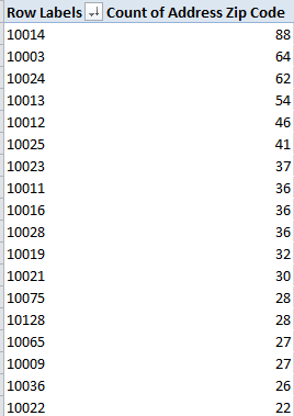
That best-in-show 10014 stands for the West Village neighborhood, a staging area for the putatively hip, followed at some remove by its opposite number of sorts, the 10003 of the East Village. It isn’t until you get to zip code 19 – 11103, signalling the heavily Greek district of Astoria, Queens – that you bump up against a non-Manhattan quarter, with its 18 cafés. In fact, 769 of the 1008 sidewalk establishments get their mail delivered somewhere on the island.
Now leave the table in place and drag Sidewalk Café Type to the Column Labels area. You should see (in excerpted form):
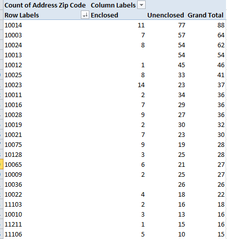
And so on. It turns out that 147, or 14.6%, of all cafés meet the Enclosed standard, officially set forth as a café “contained within a one-story structure constructed predominantly of light materials such as glass, slow-burning plastic, or lightweight metal.” In other words, if you want to catch some rays you’ll have to seat yourself somewhere among the other 85.6%.
But you want to know about those lats and longs, the better to dot your latest mapping viz. The problem is that these coordinates are beaded to those larger text expressions peopling the Location 1 field., eg.:
2 35 STREET
NEW YORK, NY 10001
(40.74910326346623, -73.98413829733063)
(The expressions are curiously formatted, perhaps having been culled from a word-processed file that lined up its text with manual line breaks.)
As a result, we need to spring the lats and longs from each such entry and plant them into cells all their own. This sort of assignment is typically entrusted to the Text to Columns feature (my January 17, post, for example), but that alternative won’t work here, in part because Text to Columns plumbs the data for a fixed set of identifiable column separators; and as we’ll see, that possibility eludes us here. But yes, there is a plan B.
To start, we’ll enter the headers Lat and Long respectively in M1 and N1. And in M2, we’ll write:
=MID(L2,FIND(“(“,L2)+1,7)
I see the board lighting up with requests for clarification, so here goes.
In fact, I introduced MID in the September 25 post, although context is everything and a second look is surely in order. MID, in contradistinction to LEFT and RIGHT, extracts a specified number of characters from the interior of a cell, and works as per this syntax:
=MID(text ,start number, number of characters)
(Where “text” can be either an actual expression or a cell reference.) Our problem is in identifying the start number of the latitudes entrapped in the expressions in the L column. What we can know is that each latitude proceeds from the immediate right of the open parenthesis (or bracket, if you’re reading this in the UK). The problem, of course, is that the parentheses debut at different locations in each entry – and that’s where FIND comes in.
Unlike MID, which captures and returns an actual textual result, FIND turns up the position of the first instance of a specified text. Thus this formulation:
=FIND(“h”,”sunshine”)
returns 5, the sequence position of the letter h. That means that our FIND nested into the larger MID expression – thus casting itself into the role of MID’s start number argument – seeks the positional appearance of the character “(” plus 1, because we’re seeking the latitude number abutting that parenthesis at its right, and not the parenthesis itself. We’re assuming of course (rightly, I think) that each and every entry in the L column in fact has an open parenthesis, and that constant empowers the formula we want to ultimately copy down the M, or Lat, column.
As for the 7, that value tells the formula how many characters to strip from the original L-column-based expression. The first three of those would be something like 40., the rounded-off latitude degree peculiar to these New York cafés, and the remaining 4 characters report the first four decimal points of the lat, e.g. 40.7491.
But once your formula is composed, you may decide that your mapping program isn’t wholly satisfied by a four-decimal latitude coordinate. That value may ground each location too finely, particularly if you’re mapping through a pivot table (October 25 and November 1 posts); and if that be the case you can brace the expressions with the ROUND enhancement, e.g.
=ROUND(MID(L2,FIND(“(“,L2)+1,7),2)
That would get you 40.75, for example.
And as for the longitudes, we need to pinpoint the appearance of the minus sign, which, unlike the parenthesis above, is integral to the longitude value (because longitudes west of the Greenwich UK, zero-degree launch point are assigned negative numbers), and as such requires us to cast off the +1 visiting our latitude expressions. Thus we’d enter in N2:
=ROUND(MID(L2,FIND(“-“,L2),7),2)
Assuming you’re content with that two-decimal point round-off. Then copy down the column.
But if you want to play with varying decimal round-offs, you could designate a cell, eg. P1, enter the 2 there, and emend your formula:
=ROUND(MID(L2,FIND(“-“,L2),10),$P$1)
That rewrite would free you to enter any substitute value in P1, say, 1 or 3 or whatever, and realize assorted precisions, e.g., 40.7, or 40.749.
But It’s coffee break time, my treat. Let’s meet at a café somewhere in 10014, your choice. You have 88 options.

Leave a comment