Marathon Data, Part 3: A Matter of Time(s)

It’s the marathon we’ve been considering but it’s raised some hurdles en route, even as we seem to have risen above them without skinning our knees. And now that we’ve handcrafted our gender variable –to look back at one of those hurdles – we might as well mix it in a pivot table or two with some other ingredients, and season to taste.

We could, for example, see what we shall see about the distributional relation between gender and age category, as our data understand that latter attribute, e.g.

18-39
40-44
45-49
50-54
55-59
60-64
65-69
70+

You’re wondering – with good reason – about that 18-39 interval and its anomalous 21-year wingspan, its incongruity underlined by runners’ overwhelming representation in that most spacious category. Try, simply

Row Labels: Category
Values: Category (Count; it’s a text field, after all)

55% of the competitors converge inside the 18-39 bracket, with no drill-downs in sight. To coin a phrase, you can’t always get what you want. And note the invisible count for blanks, because by definition category-less records have no data to count. But what about a gender proportioning of the runners by age?
Steer Gender into Column Labels and swap Gender for Category in the Values area, because the former field is wholly populated, and hence thoroughly countable. Click PivotTable Tools > Options > Show Values As > % of Row Total and:

I’m moderately surprised. The data limn a near-straight-line association between category and gender (excepting the blanks, an interesting discrepancy); female participation droops with age, and, demographics being what they are I would’ve have supposed quite the opposite. Crudely line-charted, I get

The story angle’s all yours, journos.
And while we’re at it, what about split differences reckoned by age and gender?
Row Labels: Category
Column Labels: Gender
Values: Split Pct Difference (Average)

That’s interesting too. Women match their marathon halves more closely than men across the age gamut; and how that might square with women’s relatively slower times is something to be thought through. This one’s for you, sports physiologists.
And for some breakouts driven by runner country? Again, no field devotes itself to nationality alone, but the data are there, packed alongside runners’ first names in the Name field in what appears to be a constant position following the name. As such, we can open a column to the right of name (that’s G in my workbook), dub it Country, and enter in the next row down:

=RIGHT(SUBSTITUTE(F2,”)”,””),3)

And copy down the column. That’s “” and not ” ” grazing the closed parenthesis in there, and it imparts a character of no length, if that’s not too metaphysical. Put otherwise, we’ve effectively deleted the ) character (for a review of SUBSTITUTE, see my May 17 post). The expression above exchanges the closed parenthesis trailing the three-letter country code for that “”, delivering, for example:

Laura J (GBR

And once that reformation is effected a simple RIGHT procedure shaves each entry’s last three characters, and brushes them into the Country field.

That looks good, but in the course of vetting our new country data I tripped over a thimble’s worth of records naming countries that you won’t find anywhere in your atlas. For example, Stuart Richard McDonald (overall place finisher 22182) appears to hail from a country called ard;

You see what’s happened. A shard from Mr. McDonald’s first names has splintered into the Country field, with GBR joining a country club – that is, the Club field. It’s a data entry misstep, but if to err is human, the repair calls for a formula. I’ll try this rewrite:

=IF(RIGHT(F2,1)=”)”,RIGHT(SUBSTITUTE(F2,”)”,””),3),RIGHT(SUBSTITUTE(H2,”)”,””),3)

That one seems to work. The formula asks if the final character in the F cell data is that closed parenthesis. If it is, proceed with the first expression as we detailed it above. If it isn’t – that is, if the closed parenthesis sealing off the country code has gone missing – look to the H column instead and execute the RIGHT/SUBSTITUTE routine there; and you could finalize the process by putting a Paste Special > Values through its paces to cut back on the byte count. And now you can break out the numbers and names by country, too.

And there’s another data curiosity making a rightful claim on your attention. You may have been drawn to the unrelieved pound signs (or hash marks, to you Britons) obtruding upon the DNS field (don’t be diverted by that field name; the data comprise runner split differentials expressed in time terms), here and there:

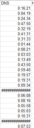
The pound signs won’t be relieved by a column autofit; rather, they hint at a mathematical impossibility of sorts. Because the numbers in effect express chronological time-of-day data, an outlaw consequence of the time format (see last week’s post), negative splits – in which second marathon halves are run more quickly than first –register an inexpressible negative time of day. You can’t have that in this cosmology, and hence the pound signs. If, however, you format the column in standard Number terms, actual usable negative numbers emerge. Just one of those spreadsheet things.

And here’s something else to look at. If you sort the data in the Split Pct Difference row smallest to largest – thus heading the column with the runners whose second halves were comparatively the fastest – the splits get rather interesting, starting with Makaela Alison Papworth, a woman whose 30,579th-place finish belies her first split of 4:00:02, a mere warm-up for a second half of 1;28:38. And if you can’t explain that 63% reduction neither can I. Let’s hope the race officials did.

And then there’s Jason Scotland, he of a first split of 2:45:15 and a second of 1:19:09. And if that sounds dodgy consider that Mr. Scotland, running in this year’s marathon as Scotland-Williams, appears to have smashed that personal best, breaking out times of 2:07:05 and 1:01:42 – the latter hurtling him into world-record territory. But in between – that is, in the 2013 race – he checked in with splits of 2:24:09 and 4:59:45.  Have we reached the limit of the benefit of the doubt, yet?

What do you think, Ms. Papworth?