Air Traffic Data: Some Reservations, Part 1

Stop me before I pun again. It’s the data’s fault, you see, a sheaf of multi-sheet dossiers of yearly traffic data for European airports and airlines, all embarking from the anno.aero site (there’s a new domain for you, or at least for me), and just asking for a jetstream of non-stop wordplay… but I thought I told you to stop me.
So let’s cut to an actual workbook – fast. Have look at this one:

european-airlines-traffic-trends

 Three sorts of sheets are loose-leafed into the book: breakouts of passenger numbers by airline and month for a particular year (the Pax) sheets, monthly percentage passenger comparisons (presumably compared with the corresponding months from the previous year in the vly sheets; and no, I don’t know what that means either), and monthly/airline figures for load factors, a measure of passenger capacity against a miles-traveled factor (see a definition here), and sheet-coded LF.

Note first of all the obvious watch-this-space vacancies in the 2014 sheets; I’m not sure why they’re presently there at all as a consequence, but note as well the column of links to respective-airline data in Q peculiar to the 2014 sheet alone, perhaps lying in wait for the folks in IT until year’s end, when the numbers finalize. Cut then to the 2013 PAX sheet and think about the workbook’s prevailing custom numeric format, e.g. as registered in cell B5:

That zero acts to round off such numbers as require it to decimal-free status, but the data here appear resolutely whole-numbered in any event, and as such would appear to have no need for that contingency plan. Do fractional passengers have to pay full fare?
But it’s the format’s defrocking of commas that’s the more bothersome fillip. Is clarity really better served by those insurrectionary spaces driving seven-digit numbers apart? And there’s an additional, more substantive quarrel to be had with the format. The first of its pound signs (or hash marks, to Britons) deals a kind of wild card to its numbers, i.e. that sign stands for all the digits that might proceed to its left (remember our numeric notation is Arabic) – and these wouldn’t be appropriately spaced, even where a space might be expected to appear. That means, for example, that if the entry in B5 were in fact

7,899,653,000

the format will redistribute it thusly:

7899 653 000

Probably not what they had in mind. (For a thoroughgoing treatment of customized numeric formatting consult this review.)
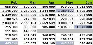
And a spot-check of the sheets snags a few other spotty design and format elements, for example the gray fills streaming across some, and only some, of the blank cells in the 2012 Pax sheet:

I can’t explain the fill’s intermittency, nor can I explain the incidence and white-font format of the formula in G14:

=(2762922-1872434/2)

Embed a white font in a white cell and you get a result that can’t be seen.
In fact, if you F5 your way to the Go To window and proceed to Special > Formulas, you’ll emblazon in blue every formula-sporting cell in the sheet, some rather unexpectedly placed, and some heretofore invisible like G14:

It gets murkier. Try F5 on the next-door 2012 vly sheet and:

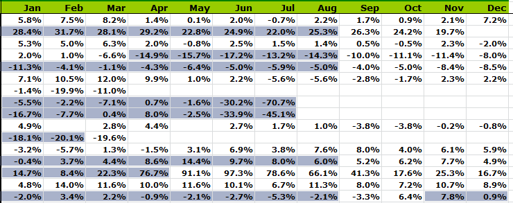
Each shaded cell sits atop a formula, leaving us to again account for their unshaded confreres. Why are some, but not all the cells invested with formulas?
And what are those formulas doing, by the way? They’re computing monthly traffic changes by airline from 2011 to 2012, performing a couple of VLOOKUPs on the data that track down month/airline numbers in the two sheets, subtracting 2011 from 2012, and dividing by the former year to stoke the percentages. Now consider the D$3 recurrently referenced in the formula strung together in D6, for example:
=(VLOOKUP($A6,’European Airlines 2012 Pax’!$A:$N,D$3,FALSE)-VLOOKUP($A6,’European Airlines 2011 Pax’!$A:$N,’European Airlines 2012 vly’!D$3,FALSE))/VLOOKUP($A6,’European Airlines 2011 Pax’!$A:$N,’European Airlines 2012 vly’!D$3,FALSE)

It points to one of a bank of hidden values (i.e. green numbers made to disappear into green cell fills) ranging across C3:N3, each one naming the lookup column number of the month below it in row 4. Thus in our formula the D$3 returns 4, directing the lookup to find its appointed value in the column topped by February. It seems to me that a rewrite might instill a quantum of elegance to the matter, by dropping MATCH into the mix in lieu of that D$3, e.g, for the first term of the formula:

=(VLOOKUP($A6,’European Airlines 2012 Pax’!$A:$N,MATCH(D$4,$A$4:$N$4,0),FALSE)

(For a run-through of MATCH look here. MATCH identifies the position, conveyed in numeric terms, of a searched-for value in a single-columned range or array. In the instance above, MATCH finds that the entry in D4 – February – is 4.)
You’ll ask what’s elegant about a replacement expression that has the effect of actually lengthening the formula. It’s elegant, I’d rebut, because formula now engages with, and only with, the air traffic data themselves (i.e. the row of month names). The numbers in row in D3 superimpose a layer of lookup values that we see could have been derived instead from the information as it already stands. But that’s just one man’s opinion.
But now what are we to make of this formula, in F12?

=(‘European Airlines 2012 Pax’!F12-258267)/258267

Or this one, in J20?

=’European Airlines 2012 Pax’!J20/’European Airlines 2011 Pax’!J28-1

Spread out before us, I think you’ll agree, is a most curious spreadsheet, its data subject to all manner of formulas irrigating a tract of cells in which formulaic uniformity would seem to be the necessary rule. It is a near postulate of spreadsheet construction that ranges of cells doing the same kind work should boast the same kind of formula, apart from the standard allowance for relative cell references. Yet the formulas here are strangely inconstant – in cells when there’s a formula to be viewed at all. That F12 expression, among other things, references the April 2012 traffic for BMI British Midland Air, but the corollary number for 2011 appears to be there, and thus available as a cell reference, in that sheet’s F17, and that number isn’t 258267, either. Yet the F17 value isn’t used, and I don’t know why. As usual, I am happy to be reeducated.

Note, by the way, that nowhere am I impugning the worksheet’s math in any of this; that is, I’m perfectly prepared to endorse the accuracy of the actual air traffic numbers that fan across the sheet (granted, I’ve yet to be asked for an endorsement). It’s how they got there, in their heterodox modes of transport, that’s the puzzler.

Not bad numbers, but odd form.