The line between instructive reiteration and a point insufferably belabored may be molecularly slight, but I’ll take my chances with your judgment and go ahead. There are, again, two types of spreadsheets: ones to be perused and read with a passive regard, and ones to be analyzed, and pushed and pulled about for some new, information-gleaning end. The anno.aero data in our collective sights must, as they’re presently organized, answer to the first criterion. After all, the spate of inconsistencies flooding the sheets won’t matter if the reader simply needs to know what’s up with air traffic numbers and move on. Maybe.
I’m equivocating even here, because similar data suited up in different clothes can give pause, even to readers happy to give the data the barest minimum of attention. I’m thinking about the Var. field at the back end of the european-airlines-traffic-trends LF (load factors) sheets, which do nothing more than subtract the previous year’s airline-specific LFs from the ones in the given year’s sheet.
Check out, for example, the 2012 LF sheet’s column P, and its alphabetically apt pp format:
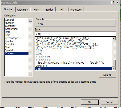
We learn first of all that Excel happily attends purely textual addenda with its numeric entries, as per the screen shot. Move into Format Cells > Custom, type a 0 in the Type: field, and tack on the text you want. (That 0 is a code representing a numeric entry). Cells subject to the makeover thus receive any numbers along with their alpha paddings, and with no loss of quantitative value – a very good thing to know, and good for me, too. The question here, though, is what the pp – abbreviating “percentage points”, I think – is doing for or with the numbers. I’d allow that, because the actual numbers in the column simply report an absolute, subtracted percent change in load factor from 2012 to 2011, the designers wanted to stave off the impression that the figures stand for some divided result, e.g., 2012/2011-1, or some sort. That’s a sage clarification on their part, but apart from a coarse rounding off of the values (the number in P4 is closer to .42% than the reported 1%) the numbers are simply hard-coded; that is, they were simply entered, sans formula. Except for the result in P22, that is, which emerges from a
=O22-B22
calculation.
And what deepens my puzzlement, though, is the Var. field in the 2011 sheet:

Those +/- 0 entries are labels, and in view of the fact that real, determinate values could have issued from the data via simple cell subtractions I don’t know why they’re there; and in any case we don’t see these labels in the 2012 sheet. Load Factors for 2013? They’re not there, even though with the contributory data in place, they could have been.
Now for something completely different but problematic: open the anno.aero svid calculator below:
(Sorry this wasn’t made available sooner.) The sheet sires a kind of cousin metric to standard deviation, measuring the monthly traffic variability in a given airport’s traffic and culminating in the index in D19 (the readings in F19 and H19 work with demo data). Note first of all the hidden E column and its operative formula, e.g.
=((100*D5/(D$17/12))-100)^2
It seems to me that
=AVERAGE(D$5:D$16)
might properly replace the (D$17/12) term, by overwriting the hard-coded 12 value (formulas respond to data-entry contingencies; the number 12 can’t), and I think the expression’s outermost open parenthesis and a corresponding closed one following the 12 could be safely banished.
The calculator asks the user to paste traffic data from one of the sheets drawn from one of the links stowed beneath the calculator (the American traffic link doesn’t work, by the way; you’ll need to divert to the anno.aero database page directly for those data); but note that the data therein are planed (sorry!) horizontally, even as the calculator wants them oriented along the vertical. As such, you’ll need to hurtle through a Copy-Paste Special-Transpose hoop, one that could have been cleared from the process.
But it’s the formula in D20 – the one that returns the textual airline rating – that’s the grabber. It reads:
=IF(D19<$A$24,$D$23,IF(D19<$A$25,$D$24,IF(D19<$A$26,$D$25,IF(D19<$B$27,$D$26, $D$27))))
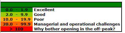
It’s nesting a series of IF statements, each assessing a value falling somewhere between the numbers in A23:A27. (Note, by the way, the space poking between the $D$26 and $D$27 references at the back end of the formula. I didn’t know you could do that.) Now if you’re wondering why the iterations above, which propose alternative after alternative in the event the number in D19 meets or fails to meet each logical test, couldn’t have been emulated by a garden-variety VLOOKUP formula I share your curiosity, but there’s a reason – sort of.
The reason is supplied by the isolated > sign, nothing but a label all by its lonesome in A27, and in a range otherwise populated by values (those hyphenated constructs, e.g. 0.0 – 1.9 – pull across three different cells; only the 0.0 finds itself in A23). And because that “greater than” is there, VLOOKUP can’t work with it. Thus the sheet designer plumped for the formulaic plan B above.
And if you doubt me, consider this excerpt from the formula:
IF(D19<$B$27,$D$26, $D$27))))
All the other IFs in there test values in A23:A26, but suddenly we’re testing a value in the B column – B27 – because that’s where the actual, quantifiable, 100 sits – and because that’s where it is, it can’t contribute to the lookup column in A. And that’s why that flurry of IFs jam the formula.
But I’ll continue to allow that a VLOOKUP will work, particularly once you scan back a couple hundred words, and rethink that pp numeric format we reviewed all the way up there. If you click in A27, return to Format Cells > Custom, type >0 (again, the zero is a coded placeholder for a numeric value) and ratify it with OK. Then simply type 100 in A27, and you should see >100, in all its adorned but value-sporting glory. Then enter
=VLOOKUP(D19,A23:D27,4)
in D20. Now when and if you paste air traffic numbers into D5:D16, you’ll evoke the same textual results evoked by the IF-laden formula (you’ll also note D20’s text-resonant, colored conditional formats).
I like that solution, if I do say so myself. As a matter of fact, I may even email anna.aero about it. And I’ll even accept frequent flyer miles in lieu of my customary fee.

Leave a comment