Last week’s run through the London borough data workbook directed its eponymous scrutiny at a fleet of VLOOKUP formulas in the book’s Profile sheet, ones that retrieved a trove of per-borough attributes, e.g. its migrant population and employment numbers. We proceeded to ask after the decision to draw the LOOKUPs’ index number (the function’s third argument, the one that returns the “answer” to the LOOKUP’s query) from a range wholly external to its table array. And here’s case in point number two on the problem.
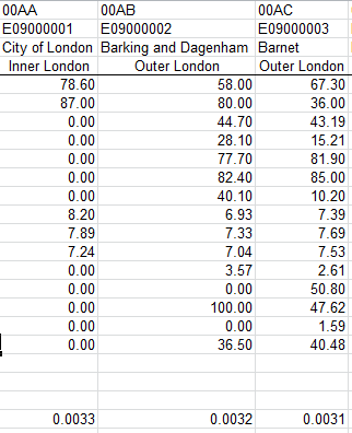
The book’s Chart-Map sheet, chief among its elements a smartly responsive cartographing of the boroughs by its user-selected attributes, binds its color-coded breakout to the VLOOKUPs in the adjoining, borough-populated range A5:B42, its second column dialing into the data array set down in the heretofore-hidden sheet, the no-less-eponymous Sheet1. The problem – again – is with their index numbers, supplied in the sheet by the invisible gray-on-gray entries in Chart-Map’s Z5:Z42 (I’ve recolored the values below in a more forthcoming white):
![]()
(The inessential decimals, nowhere to be found in the referenced cells whence they came, likewise remain to be explained; but that isn’t make-or-break, we’ll agree.)
Again, precisely the same question could be asked of the formulas here that we asked last week; they’ve keyed their operation to a range of proxy index numbers that could have, and really should have, been drawn from the table array itself. The reasons why were recounted in last week’s post, in which I filed my brief for the array’s independent, self-capable knack for returning index numbers, provided you’re on speaking terms with MATCH and like functions. (In addition, the Chart-Map’s T5:Z61 region – all of whose cells wear the gray-on-gray mask -hides all kinds of referential data, much of which undergirds the workings of the map itself.)
All of which tilts the slope towards the next question. As with the Profiles sheet we tangoed with last week, Chart-Map hangs its mapped results atop a drop-down menu comprising the seventy-or-so borough attributes on which the user can click. But it’s pipelining its core data from the Sheet1 sheet; but Profiles quarried its numbers from the Data tab instead, and it may be proper to ask why.
I’m asking why because the Chart-Map VLOOKUP for Barnet, the borough that exemplified my formulaic review last week, reads
=VLOOKUP(A$3,Sheet1!$B:$AP,Z12,FALSE)
But why couldn’t it read
=VLOOKUP(A12,Data!C:BW,MATCH(A3,Data!C1:BW1,0)) ?
To be sure, the latter expression is the more distended, but it
a) Again closes off and bats away any recourse to an external source for those VLOOKUP index numbers, and
b) Returns to the Data sheet for its lookup array – the same array Profiles used, rather than the one offered up by newcomer Sheet 1.
The question, rephrased, then: why perform lookups upon two data distinct sources when only one – either one – could execute both jobs? And by corollary, we could dare to ask if two data sets – that is, Data (and we won’t make much here of its blank row 2) and Sheet 1 – are needed at all as a result.
Click back and forth between the two. I am, as ever, happy to be brought into line, but I would allow that the two data sets are in effect equivalent, their difference a matter of orientation, with the boroughs beamed horizontally in Sheet 1 and vertically in Data, and with the borough attributes by extension pulling along the respective perpendiculars in the two sheets.
In short, the data in the two sheets seem basically, if not completely, identical, and if so – even as I can’t claim a line-by-line vetting of all the numbers – then it’s clear that one is expendable. We’re left to wonder in turn why both have been allowed to maintain their position in the workbook. I’m just asking.
I’m also asking about the formulaic involutions in lookup that restate the same borough population totals elsewhere. The totals in column B have routed their data from the same-lettered column in the Chart-Map sheet, which in turn secured its numbers via the VLOOKUPs debated above. But lookup’s (probably an infelicitous tab name, at least for our purposes) D column taps into that B data but two fields to its left, deciding in addition to test the fittedness of those values with an IF statement, e.g. for Barnet:
=IF(B6=”.”,0,B6)
Because all the data appear to be in place, I’m not certain what misgiving provoked the above formula’s search for the problem “.” in lieu of a borough’s actual population, but the misgiving seems to have been expressed; and while I’m all for leaving a spreadsheet’s formulas intact for the next person, I don’t know the contingency for which these formulas are preparing. But perhaps more to the point, couldn’t have all the formulaic toing-and-froing been overruled by a simple hard-coded, typed, references to the borough population data in the Data sheet?
And another question, as long as I’m asking: what do we make of Sheet 1’s borough population totals in the in row 5, e.g. the expression for Barnet in E5?:
=E79+E$73
First, E79 points to a data set of which I was simply unaware: a near reproduction, starting in row 75, of the data in the upper half of the Sheet1. That upper half – the half I had assumed served as the one and only data set in the sheet – simply appears to apply its ubiquitous formulas to invoke parallel data below – plus a curiously diminutive value shadowing the data in row 73:
Those entries in the lowest row above are sequenced downwards, each succeeding borough in its column receiving a decrement of .0001 – and I don’t know why. Nor do I know what the formulas above in Sheet1 bring to the analysis that the hard-coded values below don’t.
But didn’t Mr. Dylan instruct us not to criticize what we can’t understand? I’m not criticizing.

Leave a comment