Now that Super Mario has bored his way back to Tokyo, let us praise Great Britain’s mighty Olympic team, and its world’s best 67 medals, followed by the United States and its 121.
Don’t read that twice – just say hello to the New Math. Here in England, where the media put the mallets to their collective tympani for all-Team GB all the time, one’s ear had to be pressed very close to the radio for news about any athletic glory redounding to anyone else.
But ok. Two weeks of harmless sporting jingoism does wonders for the commonweal, one supposes, and so now I can tell my co-residents here that, glory aside, United States Olympic team has something the British contingent doesn’t: a spreadsheet about its members, available worldwide here:
http://www.teamusa.org/road-to-rio-2016/team-usa/athletes
Just click the Sortable Roster link.
The workbook’s name could be asked about for starters, because properly structured, any data set should be agreeable to sorting. You’ll also take note of the cell borders sectioning off respective sport (team) rosters, demarcations that no longer demarcate once one takes the workbook up on its offer and actually sorts the data by say, Last Name or Height. Because the borders will remain exactly where they were drawn – even when the sorts reorder the records – they’ll now be bordering near-random assortments of athletes.
But now to the data. The Team USA site lets us know that 124 of the team’s 558 members, about 22%, are California-born, an impressive disproportion over and above the state’s 12% contribution to the American demographic whole. If we want to break team representation out by all states, then, a pretty straightforward pivot table should be up to that task:
Rows: Birth State
Values: Birth State (count)
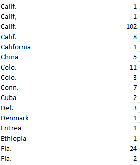
Straightforward, but problematic, e.g. this excerpt:

We’ve seen this before, and now we’re seeing it again. The Olympics may encourage diversity, but promoting disparate spellings of the same state name is grounds for a DQ, at least in this event. Note the pairs of Calif., Colo. and Fla. in the screen shot, a spate of duplications (and there are others in there) inundated by superfluous spaces. Note as well the misspelled Cailf., and it seems that full attention hasn’t been paid to the business of getting the data in shape.
But that’s where we come in. First we can sprint over to column R, the free column alongside the SCHOOL/COLLEGE. The rows in R seem to have been formatted as Text, and so I clicked the R heading and redefined the column in Number terms. Then in R2 I entered, simply:
=TRIM(L2)
And copied it down R, selected and copied those results, and pasted their values atop the L entries. (Having discharged that remit you could then go ahead and delete the contents of R.)
That standard corrective works, so far as it goes, but it won’t respell Cailf. That kind of repair might require a record-by-record edit that could make washing your socks seem exciting by comparison, though I for one would opt for the former activity (and discrepancies notwithstanding, I also get just 113 Californians, 111 if you break the residences out by the Current State field instead. I’m also not really sure what distinguishes Hometown State from either the Birth or Current State identifiers). But if you do need to know about team-member state origins (and non-American birthplaces as well), this kind of work just has to be done. Sorry.
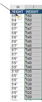
And what about athlete weights, a numeric metric that could be productively associated with sport, height, and gender, and perhaps even date of birth? Don’t be disconcerted by the left alignments, but here too we meet up with an issue – namely the more than 50 weights that sport (ok – pun intended) their values in text format, tending to cluster among the Rugby, Gold, and Equestrian members, by the way. But this gremlin is easily sent on its way, however; sort the field by largest to smallest, thus packing all the text data at the very top of the field. Select the problem data in I2:I56 and click the attendant exclamation-pointed notification:

Click Convert to Number, and the weights acquire real, measurable poundage (note the weight and height for gold-medal swimmer Ryan Held are missing).
But what about the Height data? The metaphor may grate, but the entries here are squarely interstitial, purporting quantitative information in wholly textual mode. As expressed here, 5’11” is nothing but text; if you want that datum to assume a useably numeric form this recommendation asks you to convey the above height in its cell as 511 instead, and impose a custom format upon it that interposes those apostrophes between the “feet” and “inch” parameters. Either way the entry is really 511, and that value may not work with your aggregating intentions. Another tip would have you enter a height in inches – in our case 71 – and formulaically dice the number into a foot/inch appearance, which again nevertheless ships the data in text status.
In any case, we need to deal with the data as we have them, and I’d allow the simplest intention is to get these labels into numeric mode, i.e. inch readings. In that connection, I’d return to column R, title it Height in Inches or some such, and enter in R2:
=VALUE(LEFT(H2,1)*12+VALUE(MID(H15,3,LEN(H2)-3))
To translate: the formula commences its work by detaching the first character in H2 – a 5 (I’m working with the default arraying of athlete records here, the first of which posts a height of 5’11”), and ascribes a numeric value to it via VALUE, supported by the given that all foot-heights should comprise one digit. That result is next multiplied by 12, yielding 60 inches thus far. I then isolate the 11 in 5’11” by applying a MID function to the task. The LEN(H2)-3 argument that registers the number of characters MID is to extract from the entry in H2 reflects the fact that any entry in the H column should consist of either 4 or 5 characters, e.g., 5’11” or 5’6”. Subtract 3 from either count and you come away with either 1 or 2 – the number of characters MID needs to pull from the entry in order to capture its inch value. Thus in our case we can add 60 and 11, culminating in 71 inches for the archer Brady Ellison. Copy the formula down R and eliminate the decimals, and our heights should be ready for the next round of analytical moves.
Almost. It seems my post-copy vetting of the height-in-inches data in R reports more than a dozen #VALUE! notifications – because some of the heights in the H column look like gymnast Kiana Eide’s 5’3, or indoor volleyballer Thomas Jaeschke’s 6-6. Neither reveal an inches punctuation, and Jaeschke’s height buys into a different notation altogether; and my formula can’t handle those discrepancies.
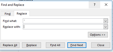
So it’s time for a Plan B. First run this find-and-replace on the heights in H:

(That is, replace the inch quotes with nothing.) That pre-formulaic fix should eliminate all the inch punctuations, directly exposing the inch numbers to the right of the cell. Then in R2 write:
=VALUE(LEFT(H2,1)*12+VALUE(RIGHT(H2,LEN(H2)-2)))
What’s changed here is the latter half of the expression, which now splits 1 or 2 inch characters from the right of the cell, depending on the single or two-character length of the inch totals. Copy this one down R and we should be in business.
Not. Two utterly obstinate athletes, field hockey aspirant Jill Witmer and soccer teammate Lindsey Horan, feature a single apostrophe beside their inch figure, a miniscule disparity that defeats my best efforts at a global formula rewrite – along with the data-less Ryan Held. Here discretion trumps valor – I’d just delete the incorrigible apostrophes and Held’s #VALUE! message, and take it from there. Now I have real heights.
Ms. Witmer – or whoever entered her data – sure is playing hockey with my fields.
Leave a comment