Granted; the line between an iconoclast and a smart aleck is but a few pixels wide, and so it’s not impossible to plant one foot on either side of the characterological divide. And while I’m straddling that gossamer border I’ll voice the notion, something at which I’ve hinted before: that Excel can do some things that other people do by mustering what feels like heavier artillery. That is, even as some practitioners of the programming arts unleash charts and vizzes of no mean quality upon their blogs, I’ll suggest in a whisper that highly reasonable facsimiles of the above can be emulated by Excel.
I’ve intimated as much before, e.g. my previous post, wherein I framed a scatter plot dotting NBA players’ offensive-to-defensive margins that successfully (if I do say so myself) imitated the chart synthesized by a corps of programmers applying a language or two (ggplot2) to the task. You may also recall my Excel-driven approximation of the celebrated charts of disease eradication here; and now I’m at it again.
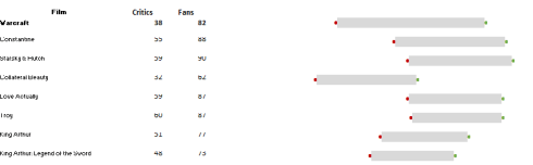
My model this time is the chart shaped by the graphics adepts at the BBC that positions the respective film ratings of critics and viewers of 2017 Oscar-nominated films, e.g in excerpt:
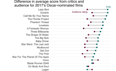
Audience evaluations are captured by the red dot with the greenish speck symbolizing aggregated critics’ scores, and the interposing gray bar conveying the scope of the discrepancy between the two assessments.
It’s a neat representation, one redolent of the controls you’d slide across this or that hi-tech contraption, though of course – excuse the iconoclasm – you could ask if the above visualization delivers its message more crisply than an off-the-shelf, industry-standard column chart that treats each film to a pair of comparative bars.
But that judgement aside, a surmise followed on: could I do something similar in Excel? I suspect you know the answer.
First, the data, which was gleaned from the Metacritic site that compiles review scores. Not being able to contrive out how to access these directly I simply transcribed the numbers from screen shots of the two sheets bearing the figures, e.g.
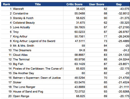
There are indeed two sheets – one reporting movies having received relatively more favorable critic ratings, the other enumerating the ones for which audience scores were the higher. In practice for our purposes, of course, only one sheet is required; there’s no operational reason for parting the sheets on the basis of the critic/audience margins.
Moreover and as you see, the screen shots feature the critic/audience rating gap for the movies, a differential that, for our charting intentions, is irrelevant. After all, the intervening gray bar should portray those differences as a matter of course (it appears by the way that some of the critic-preferred subtractive differences aren’t quite correct).
For the sake of demonstration I then simply transcribed the data onto a spreadsheet for 20 records (say A4:C24, reserving the top row for headers) – ten in which critics’ estimations topped the popular appraisals and ten in which the support trended the other way, and rounding off the numbers when required in the interests of demo simplicity.
I then selected D5:CY5 – thus bridging the 100 columns following C and so making room for any potential audience/critic rating – and proceeded to clip their widths to .42 (a measure on which you may want to experiment), and entered in D5:
=IF(OR($B5=COLUMN(D5)-3,$C5=COLUMN(D5)-3),CHAR(149),0)
What is this formula doing? First, it needs to subtract 3 from each column reference (COLUMN identifies the column number of a reference, e.g. =COLUMN(D4) returns 4) in order to for D5:CZ5 to span values 1 through 100. It then asks if a given cell’s column value equates to the film rating stored in either B5 or C5; if so, the qualifying cell(s) (one of which should satisfy the stipulation in B5, the other in C5) installs a dot, via the CHAR(149) expression, the character number for that symbol in Calibri. And that’s a dot, not a sentence-capping period. (Note that I’ve elected to size the dots to 13 pts, given the column widths, a reading you may want to tweak.) I then copied the formula across D5:CY5.
In view of the tact that my first film – the one I recorded in row 5, Warcraft – received an average 38 ranking from critics and a boffo 82 from filmgoers, the dots should instate themselves in positions 38 and 82 – in default black. A hip color, perhaps, but we want to emulate the green and red buttons the BBC set forth – the green for the audience rating, and red for the critics’ assay. That sounds like a job for a couple of conditional formats; and so after selecting D5:CY I can write
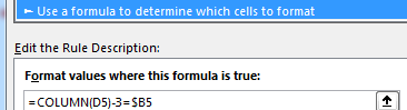
and
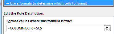
These expressions ask if any cell falling within D5 and CY5 equals the value in B5 – the critics’ rating – or C5, that of the general viewers. If the former condition is met the dot turns the critics’ red; fulfillment of the latter logical test colors the dot green. Note that because the CHAR(149) realizes a textual result – that is, the dot is just that and not a conditional formatting icon – the conditional format invokes a font color change.
Now we next need to engineer the gray band that connects the dots, as it were. I selected D5:CY5, and fired up another conditional format formula:
=AND(COLUMN(D5)-3>MIN($B5:$C5),COLUMN(D5)-3<MAX($B5:$C5))
The AND statement looks for cells whose column values register a number between the respective critic and audience ratings. Cells that conform to the criteria receive a gray fill color.
And all that means that the charted scores for Warcraft look like this:

Not too bad, but I’m biased.
If you’re happy with that take, you can copy the contents of D5:CY5 down through the other films, a move that’ll bring the conditional formats along with them. Next, in the interests of presentational clarity, I’d insert a blank row between each pair of films. (If that stratagem sounds slightly tedious, see this alternative that might or might meet with your approval.)
That chore attended to, the ratings start to look something like this:
I think it’s ready for release; I may submit it to Metacritic, in fact. I, for one, give it an 84.

Leave a comment