spreadsheetjournalism

What do chess, scrabble, bingo, planet earth, and Excel have in common? Not much, save one central, jointly indispensable commonality: all of the above conceive of themselves as grids of various vastness, cubed into coordinates named by the junctions of their row and columns.

The earthly cell references are longitudes and latitudes, pinpointing the world’s intersections under the descriptive auspices of one of two vocabularies. One speaks the language of N/S and E/W, e.g., Boston=42◦21◦N/71◦03◦E, the other a language of continuum, Boston: 42.321597/-71.09115, the minuses deriving from positions either east of the Greenwich meridian and/or south of the equator.

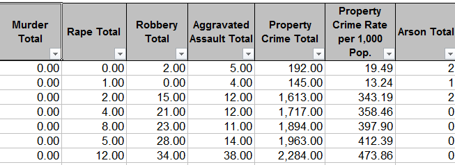
It’s the latter dialect that serves spreadsheet cartographers well, its values strung along a unitary span. And what’s to be made of all this? To begin to answer that quasi-rhetorical question, let’s return to the Washington DC crime data at which we looked a number of posts ago (August 14). We subjected the data there to a series of time-based scrutinies, e.g., crimes by day of the week and the like. But the data also plot the crimes in space, by companioning them with their latitudes and longitudes.

So here then is the plan: why not break out the data by location, lining a pivot table Row Labels area with latitudes and its perpendicular, the Column Labels area, wth longitudes? Each cell in the table, marking the crossroad of a latitude and longitude, would thus be addressed in spatial terms, and in a manner that would more-or-less respect the proportionate distances between coordinates. In other words, we could in effect literally map the data – a kind of character-based data viz, the map comprising the values slotted in their cells. Then tincture the numbers with a conditional format (the discussion of which is planned for Part 2) and you’ve heat-mapped the table.

To start afresh, you can download the DC data here:

Once accessed, the workbook-map gestates into shape pretty easily – once we get past a couple of provisos. You’ll note that the latitudes and longitudes (let’s call them lats and longs henceforth, if those abridgements aren’t too cute. But if you’re already acquiescing in the z in data “viz”, you’ll doubtless cut me this slack) are extended to 12 decimal points, in the interests of placing the data precisely at the crime scene.  But that very exactitude militates against useful data generalization. We want to able to abstract the data slightly upwards, coarsening the lats and longs into larger districts across which crime patterns might, or might not, coalesce.  When you consider that one degree of longitude in DC reaches across about 54 miles (see the web site http://andrew.hedges.name/experiments/haversine/ for some neat fill-in-the-blanks lat/long distance calculations), drilling that span down 14 decimal places will probably yield a unit measurable with a ruler.

As a result, I’ll propose (of course all is changeable in these regards) that we round the lats and longs to 3 places. If I’ve done the math reasonably correctly, that’ll take us to thousandths of a degree, for longs in DC about .054 miles, or about 260 feet – still pretty drilled-down, but a workable start.  Remember of course that a simple reformat won’t impose any substantive, valuational change upon the numbers. Formatting

38.89345352158069

as

38.893

Will still preserve all those 14-decimal points, and formulas will continue to work with them. All you will have changed is the number’s appearance. Rather, we need the ROUND function:

=ROUND(cell reference,number of decimal points to round off)

a mechanism that changes the substantive value of the number being rounded. Thus if the prolix number above sits back in cell A1 then

=ROUND(A1,3)

will bring about an actual, usable 38.893. So let’s do the following: select the K and L columns, these sporting superfluous city information, and delete their contents. Then name K Lat and L Long. In K2 write

=ROUND(I2,3)

and in L2

=ROUND(J2,3)

And copy both down their respective columns (you may want to widen L in order to be able to view the 3 decimal points).

Then it’s pivot-table time. Put the table in place in drag LAT to the Row Labels area. I get 178 values spurting downwards, probably too many to support meaningful generalizations. Thus we can group the lats by intervals of .01, although needless to say you can fool around with other increments (recall that our rounding offs above acted upon individual lats. Here we’re enfolding several lats into a manageable cohort. Nevertheless, rounding itself does enforce a manner of grouping, as well. Rounding 38.9913 and 38.9911 to 3 decimals renders them identical). Click anywhere among the lat data and click PivotTable Tools > Options > Group Selection. Type 0.01 in the By: field. You should see:

Now we can move to do something similar to the longitudes. Drag LONG to the Column Labels area, and the results will bolt all the way to the GW column (is that George Washington?), rather a way-out venue. Again, click among the data and return to Group Selection and an 0.01 reading. That compresses the grouped numbers back to the V column.

Then drag OFFENSE into the Values area. You should see something like this (my shot is excerpted):

You’re starting to get the idea. We really have in effect mapped the data against their spatial correspondences; note the clustering of crimes around the -77.034/-77.024 longitude, for example, as well as the numerous blank spaces across the table, which may – probably – denote uninhabited precincts. That is to be researched, of course, but in any case the point has been established – namely that DC crimes are by no means randomly dispersed (of course a closer consideration would require a scaling of crime numbers against the populations of the locational groupings above; and by adding a second OFFENSE entry, this time to the Report Filter area, specific crime-type distributions could be bared).

Now for a final observation today on the Group Selection feature. I had recommended a rounding of  the workbook  lats and longs to a 3-decimal point bore, in order to tailor the physical spaces with which we’ve been working into what could be termed sociologically practicable sizes. But there’s another, more strictly operational reason to round off: if you toss long-decimal values into a pivot table and proceed to group them, you surrender all formatting rights to the outcome. That is, if you had grouped the native 14-decimal point values and attempted to group them, they’d look something like this:

And the point is that the hallucinogenic tableau above can’t be formatted any further. The grouping absconds with the values’ numeric status and relegates them to inoperable, inert text. If you doubt me, try formatting them.

And if you succeed, you can call me – collect.

A Bit of Streamlining

When we last exchanged business cards you’ll recall my introduction of the Text to Columns feature, a time-honored, relatively self-evident means for farming out data amassed into one cell into a set of usable columns:

But in the course of one my solidtudinous walks in the forest it occurred to me that the lines above could be drawn more sparingly:

Here the lines flank all the incipient date and time data, but this will work nevertheless; the resulting expression retains a numerical, as opposed to text, character, and as such remains friendly to the WEEKDAY, YEAR, HOUR, etc. class of time-culling functions.

Some Watchwords About the Data

By way of additional review I’ll remind you that these posts draw upon tweet downloads emanating from the www.twdocs.com site, and in the intervening week during which I’ve splashed around the data I’ve learned some additional, cautionary things which you need to know, but which can be reconciled pretty easily:

• A two-word search, e.g., Obama Romney, appears to proceed under the aegis of an OR operator. That is, you may turn up a tweet containing only one of the two words.
• For a small proportion of downloaded tweets, the searched-for term(s) may not appear at all. I’ve emailed twdocs about this curiosity, and as of this writing have yet to hear from them.

Of course these anomalies can compromise your takes on the data, but again, there’s a practicable way to deal with these loose ends. Say I’m requesting tweets containing Obama Romney. To ascertain that I’m getting what I want once the download materializes, I can click anywhere among the results and turn the Filter feature on (Data tab > Filter in the Sort & Filter button group). Click the down arrow atop the Text field and move into Text Filters > Does Not Contain. Enter:

(Had you been seeking Obama Romney as a contiguous text entry – highly unlikely, in this case – you would have entered both words in the first field.) Click OK, and you should view a small number of records remaining onscreen, their row headers colored blue. Select all the row headers, right-click anywhere among the selection, and click Delete Row. Then turn the Filter button off, and to your relief all the other records – the ones that do contain the terms Obama and Romney – will reappear. Your data will have thereby been cleaned. It’s an irritant, but a 30-second one.

 The Data

In the interests of continuity I’ve supplied another workbook built on the big data key-term search, but these data were garnered today, Much of the preliminary work, including the data sweep described above, has already been executed. You can get the workbook here:

 bigdata2

Now let’s look at some – but only some – of the things you can do with the data.

Tweets per Hour: Calculating Velocity

Once you’ve dropped that passel of tweets onto a worksheet and vetted its data character, you might want to speed-gun the results, that is, count the tweets on the worksheet and divide the sum by the length of time they took to gain a foothold on Twitter’s servers — a simple measure of topic popularity. Working with the data as they’re positioned on Bigdata2, the relevant formula looks something like this:

=COUNT(C2:C1229)/((MAX(C2:C1229)-MIN(C2:C1229))*24)

What, then, is this formula doing? It’s trading on the understanding that dates are really numbers, and as such is determining the largest number – that is, the latest date/time – staking the column, and subtracting from it the smallest number – that is, the earliest date/time. That difference is what’s divided into the tweet count. (Note: you needn’t bind yourself to the precise 1229 last-row value when penning the formulas; you can enter 5000, for example, because Excel will ignore any blank cells here.)

But what about that 24? This curious addendum to the formula acts upon the time segment of the date’s numeric equivalent. To explain:  if October 18, 2012 is rendered numerically as 41200 (the number of days distancing it from the baseline January 1, 1900), then 41200.5 stands for noon on that date – the .5 standing for half of the elapsed day. A decimal of .25, then, represents 6:00am – or the passage of one-quarter of the day. And if you multiply .25 by 24, you get 6 – 6 hours that is.  And in turn if you subtract the earliest recorded date here from the latest, you get .471794; multiply that number by 24 and you get 11.32 hours – and that’s the number you’d divide into the number of tweets. (Just remember that 6.2 hours isn’t 6:20am; it’s 6:12, because .2 of an hour is a decimally-rendered 12 minutes).

Thus our data drive a per-hour tweet average of 209.0973 (yes, you may want to scale down some decimal points).

Tallying RTs

Another metric of apparent interest out there is retweet frequency, a calculation to which our data are most amenable. (www.retweetrank.com lists the top 10 tweeters whose messages are retweeted; when I last looked Marshall Mathers/AKA Eminem  topped the league leaders. He has over 12,000,000 followers, and follows none. You can draw your own conclusions about the zeitgeist.)

Title the G column RTs, click into G2, and enter:

=IF(LEFT(B2,2)=”RT”,1,0)

(The “RT” isn’t case-sensitive, by the way.)

The formula responds to one of two contingencies: If the tweet’s first two characters are RT, a 1 will register in the relevant cell. If the RT condition isn’t met, a 0 is supplied instead. Copy the formula down the column, and in a blank cell of your choosing that’s out of harm’s way, say J1, enter:

=SUM(G2:G1229)/COUNT(B2:B1229)

What’s we’ve done here is simply total the 1s descending the G column and divide that sum by the number of tweets. I get .276059, which presents itself as 27.61% in percent-format taken to two decimals.

A Measure of Content

Once your tweet download is in place you might well want to prospect the data for key words or terms likely to predominate, or trend, across the tweets. Since the tweets circumscribe a finitely-drawn time span, this sort of evidence could be of more than a little journalistic utility.

Here’s what you can do to capture trending terms: Enter the term for which you’re currently searching, say in K1. I’ve entered the word “security” (without the quotes), but it could be anything, and the entry is always changeable. Next, title the H column TrendingTerm or something comparable and enter in H2:

=IF(ISERR(SEARCH(K$1,B2)),0,1)

To explain: this formula owes its efficacy to the SEARCH function, which inspects a cell (here B2) for a search term (the first element or argument, in this case the contents of K1). If found, the starting position of the term is returned. If the item isn’t there, the #VALUE error message commands the cell. Thus if I write

I like brownies.

in cell B16 and brownies in A19,

=SEARCH(A19,B16)

Will yield 8, the character position at which “brownies” begins (you can also enter “brownies” in the formula, in lieu of A19). I should add that SEARCH and FIND are near-twins; the difference is that SEARCH exhibits case-insensitivity

Thus our formula in H2 issues an IF statement: if the searched-for term in cell in K1 doesn’t appear in H2 and spurs an error message as a result, a 0 alights in H2. If the term is found and thus yields a starting position number, H2 receives a 1 instead.

Copy the formula down the H column (remember, you need that absolute reference dollar sign to the immediate left of the 1 in K$1). Again as with our G-column activity, a quaintly binary stream of 1s and 0s plunge down the column. Next, say in K2, enter:

=SUM(H2:H1229)/COUNTA(B2:B1229)

The formula is identical in spirit to our RT frequency calculation: it adds the H column’s values and divides the result by the number of all tweets. For “security” I get a 10.67% incidence rate, denoting the percent of all collected tweets in which “security” appears. If I replace “security” with say, “cloud”, I get 8.71%. You can obviously enter any term, though.

And once you nail that understanding down there’s no reason why you can add additional trend-search columns in I,J,K, etc., calling upon the above formulas (with appropriate cell addressing, of course). You can enter the terms you’re searching in K1, L1, M1, etc., and have the respective columns search for each. Of course “big data” has merely served as an example; this whole exercise can be applied to more provocative tweet searches.

And of Course, Some Pivot Tabling

Of course. Once the data are properly groomed a battery of possible pivot tables awaits. For example, click anywhere in the data and order up a pivot table. For starters you can

drag Date into the Row Labels area.

To start, you’ll behold something like this:

You’ll doubtless want to group these data into day and/or hour and/or minute units. Click anywhere among the dates and Click PivotTable Tools > Options > Group Selection in the Group Button group. You should find the Months parameter selected. Click it off and click Days on. You should see:

Not very differentiating, is it? That result tells you that all the collected tweets with which we’re working were composed today, bidding us to fine-grain the data. Click on the 18-Oct (or however your date is formatted), return to the Group Selection window and click Days off, and Hours on. You should see:

That’s probably more like it. Then drag Text into the Values area. You should see:

Now that’s a touch more interesting, again hitched to the need to understand the operative time zones (see Part 1).

Now for finer granularity still, drag the Minutes field beneath Date in the Row Label area. Click anywhere among the Minute data and revisit the Group Selection window. This time you should see:

For the sake of variety, replace the 10 in By: with 5. You should see (the screen shot excerpts the whole):

You get the point. Here we see tweet frequencies distributed across 5-minute intervals.

Allow me emphasize that the data run-throughs I’ve recounted here represent only some of the analytical work you can pursue, and only some of the ways in which that work can be realized. There is assuredly more you can do; hope you’re inspired to do and learn more.  As a matter of fact, it sounds like the stuff of which all-day workshops are made. Interested? Then give my agent a call.

I just realized –  I don’t have an agent.

Election years call for new and intrepid ideas, policies powered to rise above the rude hurly burly of we vs. they, consecrating their noble intentions to nothing less than the greater national good and putting the sectarians to rout. So here’s my idea: Let us tax all Americans in proportion to their Twitter following.

Fair, indubitably transparent, and toughened against all loopholes, the plan would finally redistribute the wealth of Bill Gates (8,505,521 followers) until we’d get to call it the Melinda Gates Foundation, expropriate the assets of Lady Gaga (follower count: an end-of-civilization-as-we-know-it 30,211,539), and gladden the meek and diffident Twitterers with their double-digited coteries, who’d be emboldened to slip the plain brown wrappers off their bankbooks with pride. And once implemented we’d never again have to pester Mitt Romney about his returns; we’d know. In short, economic justice at last.

But there’s more you can do with Twitter than just hammer another plank into some dreamer’s platform. There’s information sounding faintly through the white noise – at least I think there is, somewhere, somehow; and indeed, a thick catalogue of apps out there perform, or purport to perform, all manner of analysis on the billions of tweets riddling the cyber cosmos.

Now while I can hardly claim to have surveyed all of these (and you’d probably think ill of me had), but after some concerted fooling around with a number of candidates I’ve cast my vote – a provisional one, mind you – for www.twdocs.com, a free and acceptably easy, and remarkably speedy tool for downloading tweets by any key term into Excel. But the analysis writ large, requires about two-and-a-half-steps – that is, getting the data into your worksheet, and then deciding what you can learn from them. The half-step trudges between the other two – understanding what sort of data you’re about to get, and by extension, perhaps, what you’re not going to get from twdocs and Twitter in general.

Some Caveats

That is to say: the analysis of tweet traffic – the figuring of tweet (and retweet) frequencies by key term broken out by month, day, hour, minute, or perhaps even seconds, user stats, and perhaps even a bit of content analysis – is constrained in part by the number of tweets you can rightly hope to access. It appears Twitter sizes its tweet-download maximum at about the most recent 1500 (the number I’ve seen at numerous app sites), and twdocs appears to reach back to only the last week’s worth of tweets, an interval which may slim some outputs well beneath 1500, simply because the searched-for term hasn’t been invoked that often in the past seven-or-so days. Also, the results aren’t quite real-time, though they’re real close. In addition, while every tweet entry that boxes itself in your cells is time-stamped the entries need to be calibrated to the understanding that people are tweeting worldwide, so one tweeter’s 8:00am is another’s 1:00pm. (The data I download seem to lag precisely an hour behind my Greenwich time zone, which either bespeaks an hour delay or the fact that twdoc’s server is somewhere over the Atlantic. In fact and for what it’s worth, twdoc is Latvia-based; in any case you should check the data against your zone.) So, if among other things you’re interested in the rates of tweeting activity for a given topic, these data should stand you in good stead.

Keep in mind as well that you can download data for the same search item the next week, too, at which point you can stack this week’s output atop the earlier ones, and thus still accumulate a large, relatively current and continuous batch of tweets. As we hope to demonstrate, you probably want to search for terms that capture your intent as generically as possible. You can search for @obama, #obama, and Obama, but the last-named should excavate the largest set of entries, and it does. A short while prior to typing this sentence, I entered Obama (in search of a max of 1200 results) and came away with 1200 entries spanning 2 minutes and 56 seconds. Entering #obama just a bit later yielded its 1200 in 1:58:05, or nearly two hours. The twdocs engine seems impressively accurate and comprehensive.

Giving It A try

Getting twdocs to work seems pretty straightforward. After supplying the site with your Twitter identity and following the start instructions (most of which I no longer remember, truth to be told; you will in addition be asked to consent to twdoc’s access of your identity whenever you log into the site) you should be transported here:

My user experience advises me to first click the CSV (comma separated values) option (in actuality a less troublesome selection than XLS) and then to click the Latest SEARCH results for…link. You’ll be brought here:

(Note the results box, in which you can type a figure topping at 1500. Note in turn the varied format options, although again, for spreadsheet purposes I use CSV – it just happens to provide a cleaner alternative, and I’m presently bypassing the advanced options for a reason). You can basically type anything in the Query field, e.g., @obama, #obama, or just plain Obama. (You can apparently type John Doe without the modifying “   “.) Then click Go. Soon this bar should stretch itself out in the lower reaches of your screen:

Just click Open.

For illustration’s sake, I downloaded tweets subsuming the term bigdata, something of a hot topic these days (and not to be confused with bighair), and saved the results as an Excel file (diverting it from its default CSV format).Here’s the file:

bigdata

For starters, the data look something like this:

After retailoring the column widths, we need decide what to do next. At least two of the presented columns,  in_reply_to and source, seem be of no informational consequence; the id field, currently formatted in Scientific notation mode, might however have a role to play in the analysis, as we hope to show. (If you want to see the ids in their standard numeric incarnation select the entire column and click Number in the drop-down menu heading the Home tab >Number button group. Never mind the decimal points.)

A Tried and Tested Tool

Now if you’re interested in rates – i.e., tweets per hour, etc. – you most assuredly will be interested in the created_at field in column C (needless to say, you can rename the columns). The data here amalgamate weekday, day of month, and time of tweet data, and as such need to be broken out. And the instrument towards this end is none other than the classic Text to Columns options, which dices information in a cell into sections, the widths of which are your call. When all is said and done we want to have assigned weekday, day-month, hour, and minute to discrete, independent columns, the better to pivot table them and the like.

Applying Text to Columns is usually (usually) trouble-free. To start, select the C column, and click the Data tab > Text to Columns in the Data Tools button group. You should see:

Note that Excel has typed the data as fixed width, the nature of which is explained alongside the term. In fact, every expression the C column happens to be 31 characters long (that is, fixed), and appears to be cleanly separable into columns wherever a space is interpolated as we’re told above. Click Next, and you’ll see

Again, Excel has drawn demarcating lines at each space, proposing to split each cell’s data into the respective columns recommended above. But we’ve been entrusted with some discretion in this matter, and what I want to do gather the 11, the Oct, and the 2012 into a single cell instead of the proposed three showing in the screen shot. In order to realize that efficiency I’m going to double-click the lines separating the 11 and Oct, and Oct and 2012, as per Excel’s instructions:

You’ll see why, I hope. Then click Next:

Now take note of what we want to see, and what we don’t want to see. My plan is to bead together 11-Oct-2012 in the first data row, for example, a mathematical date (as opposed to text) entry from which we can then ferret weekday, month, and year if we want to. If I’ve gotten that right, then we don’t need the leftmost Thu, entry, with that superfluous comma that would have to squelched, if only for formatting reasons. But again, if I’ve played my cards right, we’ll see that the day is already folded into 11-Oct-2012, as it were. In that light I can click the column header above Thu, and click the Do not import column (skip) button, and do the same for the column sporting the redundant and ultimately useless +0000 data:

Then click Finish. You should see:

Remember we’re about to perform an act of fission, parting the column on which we’re working into two serviceable columns – and Excel in turn won’t make room for the new field(s) by inserting a corresponding set of insurgent columns. Rather, Excel will simply overwrite any data in as many adjoining columns to the right of the data as are required by the new columns. But we’re fortunate in this case; we’re halving the current column into two – and so only one existing column will be overwritten – one of the columns we don’t need: in_reply_to. Click Finish. You should see:

Now date has been severed from time. (Note by the way the original column title – created_at – has also been sundered, but that’s not a big deal. Just retitle it, and also title the new column carrying the time data.)

We’re not finished, because we still need to see day-of-week, hour, and minute fields in order to empower our analysis (I’m not providing seconds as a unit of time though the data are available; but operating at that level of precision will start to get messy here). In the E column, the one containing the extraneous “source” data, type in E2

=WEEKDAY(C2)

You should return the value 5, or Thursday. Copy that formula down the column and retitle it Day or something like it. In the vacant G column type in G2

=HOUR(D2)

And copy down the column (and title the column, too). I get 13 in G2, as I’m operating with European time settings.

And in H2 type

=MINUTE(D2)

And copy down the column (it needs a header, too).

Your workbook should look something like this:

And if you haven’t been saving the workbook throughout, save it now!

Now the sheet is primed for analysis. Let’s see what we can do with it.

In the meantime, just remember – if you stop following Lady Gaga, you’re an accessory to tax evasion.

My WordPress contract grants me a vacation every 14 posts, so according to my math now’s the time. Anyway, I’ve been working too hard and I need a break. (Did I just say that? I must have; my nose is growing.) Absent a late-breaking development I hope to be back here around October 11, though I should have email access intermittently.

Now for the addendum, a quick one. The kind of spreadsheet you want turns in large measure on what it is you need to do with it. The UN birth-data sheet I commended in the post below works as a primary research source, but clearly won’t serve a public keen to tune into recapitulated, ready-to-read results. As such, the NPP worksheet might very well speak to that public in its language.

The question, one which denominates a real spreadsheet conceptual divide, is thus one of Before and After:  is the sheet something you want to read right now, or something on which you want and need to work? I’d allow that for the story generator, you want a Before – the data backstage, 1,000 rows and 50,000 characters in search of an author.

@abbottkatz

abbott@abbottkatz.com

You’ll recall my last post (and if you don’t, just scroll down; I’ll wait) broached the not-awesomely-exciting but integral matter of spreadsheet data, their contents and their discontents – that is, challenges of working with information that just won’t cooperate with your plans to refurbish and ready it for a round of analysis pegged to your story-seeking needs. And there’s is more to consider on this count, including a recurring, foundational, spreadsheet design question you do need to think about. So prepare to be unexcited again.

The problem is pointedly typified by a worksheet I’ve carted off from

http://data.nationalpriorities.org/searchtool/

a government site that breaks out and maps various federal expenditures along a number of budgetary variables.  The one I’ve brought to your attention, a state-by-state (and US-territorial) gender census for the years 1990-2010, comes to you right here:

NPP_FPDB_PopulationbyGender

(You’ll note first of all that no data avails for any of the territories, but that’s the way it goes.)

The communicative intent of the spreadsheet is clear – to tally state populations by year and gender, and as far as they go the data are nothing if not intelligible; so if you’re bringing a casual viewer’s eye to the sheet, the tableau unfolding before you may suffice as is. But if you’re expecting more from the data, a harder look may be in order.

For one thing, the worksheet has more columns than the Parthenon, appointing female, female percent, year male, male percent, and year total fields to each of the 21 years compiled and culminating in a distended, awkward read:

Moreover, the alternation and reprising of fields, i.e., female, female percent, male, male percent, year total for any year, and then again for the next year,  inflicts a crimp in the formula-writing process – not a prohibitive one to be sure, but an irritant at the least. It would be easy enough to sum each column – say, all females for 2010 – but calculating the average female percentage by state across the 21 years, for example, would involve an expression starting (say for Alabama)

=SUM(B2,G2,L2….) and so on, to be divided by =SUM(F2,K2,P2…) and so on.

And you’d have to do something similar for male percentages. Again, these conjurations aren’t forbiddingly complex, but you’d have to plant them in column DC at best (that is, the first free column), and additional formulas grounded in the data streaming horizontally would have to lurch farther out still (one need not be troubled by all those N/As, however; those are text entries and not formula-resultant error statements, and so standard formulas will ignore them without hazard. You could, on the other hand, simply delete the N/A-beset rows, because they contain no data at all.).

Once thought through, the sheet’s presentational inelegance and impediments to productive data breakouts are problem enough; but once you decide to commit the data to pivot table scrutiny, the problem burgeons – for a very – er, pivotal – reason.

The problem – a classic one haunting this kind of work – is this: the worksheet under your steely investigative gaze has awarded individual field status to what should be more properly accredited as items.

And exactly what does that mean? It means that the year fields – all 21 of them  (these in fact hybrid fields twinned with a gender property) – could have, and in my humble estimation should have, been compliantly huddled beneath the umbrella of a single field – something called Year, or something like it. And it means that Female and Male – the attributes bolted to those 21 years – should have been spirited away and sequestered beneath a new, liberated field called Gender. In my view, the data should have been arrayed more or less like this, using four years’ worth of data in this truncated example:

And so on, down the respective columns for all the states and all the years. Now while these records appear at first and perhaps even second blush to suffer from a kind of data profligacy – after all, we’d need to enter each state name 42 times (21 years times 2), even as each was keyed in exactly once in our downloaded worksheet – yet major analytical and presentational efficiencies follow as a result, because when these redrawn data are visited upon a set of pivot tables, you can get this:

And this:

And this:

This rather abstruse formulation delivers the percent increase in men by state, relative to the preceding year – and there are notable divergences by state.

Granted, these data don’t conduce toward Eureka-level findings, but the larger point is there to be made, namely this: that data of what could be called the same order of phenomenon belong together, enrolled as items in the same field. Thus here, year data should be accounted as discrete instances, or items, of the overarching field called Year. The two genders should likewise be made to share the space plotted beneath the field Gender, or some such suitable name. And the states should not in turn be allotted separate field statuses – i.e., a field called Alabama, a field called Alaska, etc. – as indeed they are not here.

The advantages of this strategy may or may not be wholly transparent to you, but they are real, and include these:

• Extending the above example: if every year were to possess its own field status, each one would have to be dragged separately into a pivot table – and that, is after all, a drag. But gathering all the years under the Year field aegis would require only one field drag.
• If each year were to arrogate separate field status, for example, each one would have to be formatted separately once having been roped into a pivot table. A unitary Year field requires only one formatting operation, and allows its data to be immediately grouped:

Try carrying out this elementary pivot task on the downloaded worksheet. I’m not sure you can, because when two fields co-reside in the Row Labels area, one necessarily subordinates itself to the other, e.g.

Thus put two independent year fields in play and one needs to appear “first” in Row Labels, in the superordinate position; the other won’t and can’t occupy the same space, appearing only subordinately in the next Row Label column as above.

• The pivot table’s native mathematical complement – that is, the Summarize by Sum, Average, etc., and Show Values As capabilities – work directly on same-field data, bypassing any need for those calculated formulas discussed in an earlier post (September 6). For example, this little pivot table elicited from my demo data:

simply enumerates the aggregate increase in US population across adjacent years (that’s why 2007 is blank – it serves as the base year). Again, the labors required to enable this sequence if 2007, 2008, 2009, and 2010 were to hold down individual field statuses is a pause-giver.

And if you’re looking for corroboration of all this, return to that UN birth data spreadsheet I   referenced in my post on Olympic birth months. On second thought, don’t bother – just check out this shot:

You see the point – the ostinato of Albanias and year entries, both items complying with the Country or Area and Year field rubrics respectively. That’s the way it should be done.

But what then of our census data as they stand – are these workable, or grounds for another write-off? I’d suggest that some room for rapprochement could be set aside here. For one thing, and unlike the adjunct data worksheet we reviewed last post, the data themselves – the actual cell-specific entries that inform the sheet – are ok in and of themselves. One could leave the data in their as-is state and throw in some of the formulas I had suggested about 1,000 words ago. But it also seems to me that with a measure of due diligence – and perhaps not as much as you might initially fear – you could, with some sage copying and pasting, restructure the sheet commensurate with the counsel I’ve proffered above (though you’d probably want to do the copying to a completely new sheet). I managed to assemble  the four-year census demo above in about  15 minutes, so if you have reason to believe that, given the proper exertions, the data  may have something to say, the project might be worth a go.

So go.

@abbottkatz

abbott@abbottkatz.com

All due props to Josh Boldt, fighting the good fight for adjunct college instructors worldwide. It’s a dirty job, and Boldt decided he’s gotta do it.

You know these adjunct folks well.  After all, you probably owe more than half your college credits to them, those front-line staff with flat-line salaries, keepers of the peace in anarchic lecture halls teeming with text-addled, twittered-out undergrads with anything but today’s assignment on their mind. Take it from me, I’ve been there;  and just because the words “adjunct” and “tenure-track” never appear in the same sentence is no reason not accord adjuncts the full eye contact they deserve when you catch them thumbing through What Color Is Your Parachute? in the Barnes and Noble.

What Boldt, a writing teacher and freelance writer in Athens (Georgia), has done and continues to do is accrete a dynamic record of the adjunct experience via a pair of spreadsheets to which adjuncts are asked to volunteer basic workplace information on a form. Each response – comprising data such as school name and location, department, salary, contract duration, etc. – is meant to add a few pixels to the big picture of the adjunct circa 2012, which may not be terribly pretty. As Boldt puts in on his site:

This website was designed collaboratively by the new majority of motivated, intelligent, and driven academics who are struggling to use their experience and knowledge in a meaningful way that benefits both themselves and society.

The spreadsheets, one earmarked for adjuncts in the US, the other for international part-timers , might thus have some interesting things to say about this oft-bedraggled work force. You can download the US rendition in Excel form here:

 adjunct data

 (Note: While you could in principle grab the spreadsheet from the Adjunct site via an Excel web query – a capability we’ve yet to broach in this blog – my repeated tries at reeling the data in through via this route failed, for reasons not entirely clear to me. But no matter – web queries refresh their data at identified intervals, normally a cool and desirable thing. But the refresh shakes out any changes made to the base spreadsheet, restoring it to its primeval state, and that’s not what we want in any event.)

I’ve saved the sheet precisely as it looked when alighted onto my blank workbook, and as such seems to be in need of a variety of repairs:

So let’s put on the hard hat and get to work. First, if we want to put the sheet in the service of additional analysis, e.g., through a pivot table etc.., we need to delete rows 3 and 4 – they’re blank, and as strand the header row from the data beneath.

Second – and I originally missed this – we need to delete the A column; look closely and you’ll see dots or periods speckling the A cells. These are data of the most purposeless kind, and should be chased away.

Next – the header row, along with many if not all the data rows, has clearly been subjected to the Wrap Text option, a fillip to which Excel isn’t doing much justice (see above). Rather than refit individual columns to widths that would suitably befit the wrap typography, what I’d simply do is select the entire worksheet (here you should click the Select All button, that unassuming blank button to the immediate left of the A column header) and click the Wrap Text button (Home tab, Alignment button group) which is currently illuminated. By turning the effect off all the data straighten themselves out atop the floor of their cells, even as the header labels pierce the columns to their right. Note that the worksheet remains selected, and so you need only double-click any column boundary and institute a mass auto-fit across the data (true, some columns will dilate to an untenable width; these can be cinched manually). Note the data cells entries are middle-aligned – that is, they ascend to the vertical centers of their cells – but I’m not bothered by any of that, and I’d leave that effect alone.

Now we need to clear away another data obstruction. Each state’s data is topped by what could be properly regarded as a sub-heading, in which only the state’s name occupies the row. These geographical identifiers can’t properly be termed data, as they bear no information about any institution and simply subsume the records immediately below. I tried a number of quick workarounds of the sort-these-rows-to-the-bottom variety we’ve discussed in earlier posts, but because the pertinent cells are so sporadically populated I had to turn to Plan B. In the first free column – K, by my reckoning – enter a header in K2 (it could be anything – I simply called it Sort), and write this formula in K3:

=IF(COUNTA(A3:J3)=1,”zz”,”aa”)

This expression does the following: it counts the number of cells sporting any sort of data in the named range (COUNT, on the other hand, tallies only those cells containing numeric values). If the count evaluates to 1, you’ve apparently nailed a row containing a state name only. If it is 1, the formula enters the text zz in its cell; otherwise, it returns the letters aa.

Then copy the formula and copy it to the remainder of the records – only here, because so many blank cells have presumed upon the data, click in the name box (the white field to the left of the Formula Bar that typically reports the current address of the cell pointer) and enter K3:K1984 (1984 happens to be the last data row on the sheet). Tap Enter twice (the first tap selects the range; the second actually does the pasting). Then sort A to Z on column K. And guess what? You’re rudely interrupted by the “This operation requires the merged cells to be identically sized” error message, about which something obviously needs to be done. Presumably because merged cells absorb two or more cells, the sort command gets flummoxed by the resulting cell address conflations and can’t do its thing. Now, I don’t particularly know which cells are in actuality the merged ones, but I’ll just select the entire worksheet again, click the down arrow fused to the Merge & Center button (Home tab, Alignment button group), and select Unmerge Cells (“unmerge”, and its cousin “unhide”, rank as two of the most stilted verbs in the lexicon, and people at Microsoft get paid a lot more than adjuncts to come up with stuff like this). Now you can sort A to Z on K, and insert a blank row right above 1928, which is where my state labels now start (remember that state abbreviations are supplied in any case in the B column if you need them).

All of which raises the question I was afraid you’d ask: Now what? And that’s precisely the point. Take a look at the Pay Per Course field, likely to propose itself as the essential parameter in the worksheet. But the data here are so multifarious, so apple-and-oranged, that our next analytical move seems to have been checked – if not check-mated.

What to do? I’m not sure. While many of the data are standard numeric fare, many are not, and banishing the latter from the worksheet will comprise the data too dearly. Would it be possible to recondition those non-numerics into quantitative form? I wouldn’t declare the chore impossible, but you’d have to bounce some headachy cost-benefit equations off your medulla, and think hard about how you’d make over a cell like this:

There are three salary figures in that cell – informative, to be sure, but try to add them.

When the data don’t cooperate –when they exhibit snarly recalcitrance – you may have little option but to direct your attention to a more compliant workbook –in other words, break out the white flag, cry Uncle, and punt (is that what they mean by a mixed metaphor?). (You might also ask yourself, by the way, how you would have constructed the worksheet from scratch had you been entrusted with that assignment.)

But none of this should be read as an arraignment of what Josh Boldt is trying to do. He’s putting together a public record, one answerable to his intentions, not ours. That the worksheet isn’t all that analyst-friendly is a discontent I’ve superimposed on the data. The sheet is what it is. And were I still an adjunct I might dial into his site and add my own info, too.

But I need work on a more pressing issue now. I need to find out if people still say “props”.

@abbottkatz

abbott@abbottkatz.com

St. Pancras Station, London, Aug 8.

Remember the Olympics, that quadrennial competition between the world’s elite corporate sponsors? McDonald’s-by-the-Thames, Lebron and Kobe on the same team, scandal on the badminton court, wholesome sublimated paint-ball nationalism (you know, my guy ran faster than your guy, especially if you live in Jamaica) and all that?

It was in all the papers. In any case, it seemed to me that the topical concern of a previous post (August 24) – namely, the modal incidence of August-born baseball players in the major leagues – could be naturally transposed to the Olympic context. Does birth month in any way broaden or constrict an athlete’s (Summer) Olympic prospects, or is the correlation spurious, or scant?

Postscript and Prelude

But before we put the lens to the data, you recall that the August birth-month skew among ballplayers is typically ascribed to the July 31 birthday cut-off for kids enrolling in any given year’s Little League cohort. That closing date makes the August-born oldest in their admitting class, so to speak, and thus bigger stronger, more adroit in the baseball arts, and thus possessive of a sustained developmental edge.

In this regard, and you may have missed it, reader James Zhang’s September 9 comment thumb-tacked to the baseball birth-month post asks a most salient, purloined-letter of a question: what if the August birth-month differential could be more properly laid not to Little League registration policies, but rather to the simple demographic possibility that more children are born in August?

A very good question, Mr. Zhang, and it turns out there’s something to it. By peeling off birth data from a melange of sources on the net (including Vital Statistics of the US) and grafting these to equivalent-year stats from Sean Lahman’s baseball database, I got, by way of a sample:

The baseball numbers aren’t enormous (averaging about 168 players per year), but the aggregate effect is pretty evident, particularly when keyed to the 8.48% “chance”-driven expectation for August births. The conclusion then is multivariate: both national and ballplayer August births better chance likelihoods, but it is the baseball effect that pulls farther away from default expectations. In any case, a birth-month tug does seem to be in force here, something to be kept in mind.

But what then about the Olympics and its vastly more heterodox, Little League-less athlete pool? What sort of birth-month association, if any, marks the data?

Let’s see. Our data source comprises the Guardian’s spreadsheet of Olympic 2012 medal winners saved to Excel and made available here:

All London 2012 athletes and medal data

(N.B. These medal data are incomplete, the workbook having been compiled before event outcomes were realized in the Games’ last three days, e.g., basketball and the marathon. I think it would be a reach to insist that the deficit degrades our analysis, but in any event John Burn-Murdoch, who works on such projects for the Guardian, tells me the completed rendition should be out there soon. For a 2008 census of National Basketball Association player birth-months see

http://statsheet.com/blog/applying-outliers-does-birth-month-matter-in-basketball ).

Some Notes About the Book

Before we broach our question – whether a birth-month effect in any way correlates with Olympic medal success – a few words about the workbook’s design would be instructive.

• Note the coupling of first and last athlete names in column A – not the by-the-book way of handling such data, particularly if you need to sort these by last name.  That task can be dealt with even as the data stand, but the task can get messy. On the other hand of course, the names are extraneous to our purposes right now – but maybe not next time.
• The Age field could be regarded as an ever-so-slight redundancy, given the companion Date of Birth field and the latter’s enabler role in helping derive real-time athlete ages. Example: if you want to learn A Lam Shin’s right-now age, replace the 25 in cell C2 and write

=(TODAY()-H2)/365.25  (the denominator represents the average number of days per year).

Her age result – 25.97 as of today – will change daily. Then copy down the C column. Just remember to send Ms. Shin a birthday card. (Of course, this formula can fall victim to its own volatility. View the workbook in ten years and you probably won’t need to know that she’s now 36.)

• Moreover the Age Group field, impressed into Row Label service in Pivot Table 10, comprises text data, and as such cannot be further manipulated absent a concerted round of hoop-jumping. If in fact you want to group the athletes by age tranches you’re far better advised to substitute the Age field and dice the data with the Pivot Table’s Group Selection option.
• By sounding an unrelieved drone of YESes in its cells, the Medal Winner? field consigns itself to dispensability, teach us nothing. By definition, the workbook means to catalogue none other than medal winners. On the other hand of course, if you have no plans either to use these data or present the field to readers you can merely ignore it.
• Note the G, S, and B fields (Gold, Silver, and Bronze) and their fractional medal representations, the Guardian’s attempt to align overall country medal totals with the grand total of actual athlete medallists, an obeisance to team-based competitions. Thus Croatia’s Valent Sinkovic in A932 comes away with .25 of a silver medal, having competed in the Men’s Quadruple Sculls Rowing event.  These apportionments do make a certain sense, but other analytical necessities may bid you to award him one, indivisible silver.

And Something Else…

Now here’s the real problem, to which you may have already altered yourself. Remember that we want to see if athlete birth-month data stack higher for this or that month, and if so, why. But unlike the Lahman baseball records that informed our baseball birth-month post, no immediate month data avails in the Olympic workbook. However, Excel’s MONTH function enables us to do what we want, and very simply:

=MONTH(cell containing date).

Thus

=MONTH(A2)

will return the value 9 (September) for Ms. Shin. Once in place, we can copy that expression down a column, and we’re done – maybe.

But look at cell H11; the date for Mr. Zielinksi exhibits a left alignment that intimates, without quite proving, that H11 contains a text entry, which simply can’t comport with MONTH, which is looking for numerical data. Remember that dates, beneath all the formatting rouge and lipstick, are numbers (see the August 20 post), and while it’s quite possible and perfectly legal to left-align a number, the anomaly in H11 hints otherwise. To clinch the point, click in any blank cell and type

=H11*2

Don’t you just love error messages?

I can’t explain why these text entries infiltrated the larger complement of workable dates but they did, and to dangle a preposition, it’s something we need to deal with. Before we break out birth months we need to see to it that all our data-to-be in fact qualify as months.

One possibility: we could sort the DOB column by Oldest to Newest and eye the bottom of the record stack. I see 21 text-formatted, faux-date entries; and while we could return to the insert-a-blank-row-above-these-records expedient (something I’ve explained in earlier posts, including August 30), thus estranging the bad apples from the usable data (they only contribute about 2% of all records, after all), we don’t have to. The reality is that we can retrieve the months from these date pretenders, and here’s how I’d to it.

Insert a column to the right of DOB and title it Birth Month. Select the new column and select Number in the drop-down menu in the Number button group:

We’ve taken that step to insure that our results here look like numbers, and not dates. Then in cell I2 write:

=IF(ISTEXT(H2),VALUE(MID(H2,4,2)),MONTH(H2))

OK – you’re entitled to an explanation of this rococo expression, though you’ve probably managed to make some fledgling sense out of it already. The ISTEXT function, written simply

=ISTEXT(cell reference)

is invariably soldered to an IF statement, and inspects the referenced cell for its data type. If the cell comprises text, one thing happens; if it’s other than text (e.g., a number), something else happens. In our case we stipulate that if the cell evinces a text content, Excel will proceed to extract the month from the cell via the nested MID function (how that happens will be detailed in a moment); if the entry is not text, that is a number, then the formula will apply MONTH to the cell’s date/number.

And how does MID work? Its three elements, or arguments as they’re known in the trade, do the following, respectively

1. Identify the cell in which MID will perform its work (H2 above)
2. Cites the position of the character at which MID will begin to extract characters
3. Declares how many characters will be appropriated from that inception point.

Thus if I type

SPREADSHEET

in say, cell A7, and enter

=MID(A7,3,4)

in A8, I should realize the character sequence READ.

Thus for our text-date data, those data to which we want to direct MID, we see that the month segment of  text-bearing cells always situates itself in characters 4 and 5 – a good thing, because had single-digit months (January through September) been conveyed in single-digit terms (9 instead of 09) we’d have had to wrap our hands around a much stickier wicket; we’d have to have written a formula that sometimes extracts 1, and sometimes extracts 2, month characters.

(Note also that the text-date cells are expressed in European date format, in which day of month precedes month, even as the other data appear in American, month-first style).

And finally, we need to brace MID with the VALUE function because our results would otherwise remain text, and we want the resulting month extraction to hold numeric status.  VALUE simply mutates a number formatted as text into its quantitative equivalent:

=VALUE(A7)

would realize the value 7, had you entered a text-formatted 7 in the cell.

Now that you’re panting from all that heavy lifting, kick back and smoke ‘em if you’ve got ‘em, because the rest should be a comparative day at the beach. Copy the formula you’ve inscribed (and you need all those parentheses in place) in I2 down the I column and you should be treated to a medley of values ranging from 1 to 12, something like this:

(Ignore the decimal points if you see them; they don’t matter.) Next, let’s pivot table the months. Boot up a table and

Drag the Birth Month field to the Row Labels area.

Drag Birth Month into the Values area. Click in the Values area, and in turn click PivotTable Tools > Options > Summarize Values As > Count (the data have defaulted to Sum simply because they are numeric). You’ll see:

I’ll take a wild guess and allow that the largest birth month happens to be…August, the only one stepping up to three figures. Note in addition the no-less-striking, precipitous fall-off in the succeeding months.

Now remain in that field and click Options (if necessary) > Show Values As > % of Column Total (again, I’m directing you through the Excel 2010 interface). You should see:

August rules – again – but of course a satisfactory accounting awaits.

Now there is some evidence for a global August birth predominance, but a closer look is clearly in order. A UN international, country-by-country birth-month spreadsheet (click the small download link, but there’s some hoop-jumping required here in order to whip the data into shape) shows a July-September birth skew, but you’d have to toil to reconcile Olympic countries and team size with these data.

Note as well that if you swing the Country field into the Report Filter area and click on United States of America (athlete total here: 120) you’ll get

Still another win for August, albeit for a relatively small universe. Another remarkable stat: filter for People’s Republic of China and you’ll behold a 23.68% birth contribution from January (athlete total: 76), an extraordinary outlier I’ll leave to the Sinologists.

Sure there are other pivot table permutations to be crunched (you could break out for gender, for example, and sport), but the principal research remit is already out there: tracking and explaining the birth-month curve. An artifact of fertility trends, or the consequence of subtle, worldwide athlete recruitment protocols – or a bit of both?

Well, there’s your assignment, and I know you can handle it. It’s why, after all, you make the big money.

The Plot Thus Far

You like to tweet? I like to tweak. Before I so rudely interrupted myself with that simpering apology below, the one about which you remain undecided, you’ll recall we spent the better part of the first installment (even farther below) assaying the King County crime-tracking spreadsheet, with the intention of reframing it for a new set of purpose-driven looks at the data. Again, the practice of emending someone else’s data needn’t always be construed as a headlong critique of the original; rather, the overhauls we want to carry out here should be read as an attempt to personalize the data, so to speak. If you’ve yet to download the workbook you can do it here:

KC crime rates 1985-2011

(You should then review the data modifications we enacted in Part 1.)

Picking up the sheet, then, at the point at which we had left it at the close of Part 1, another perambulation across the data yields 20 records (at least that’s what I get) whose Months Reported amount to fewer than 12, or in other words, less than a year’s worth of data. Of these, four rows offer up 0 months, meaning that, for whatever reason, there’s nothing here to report – no crimes, nothing. Leaving aside the reasons for that data dearth, I’d sort Months Reported descendingly and jam a blank row immediately above those zeroes, thus isolating them from the substantive rows.

But those remaining, fewer-than-12-month rows need to be thought about, and thought through. After all, these 16 or so records do divulge crime data, but because their totals are necessarily fractional we need to extrapolate these to an entire year. For example – the Index Crime Total (the sum of all reported crimes) in column E for Algona in 2004 shows 40 for its nine months’ worth of tracking; but 40 doesn’t represent a rate, but rather an absolute figure, and as such needs to be mapped to 12 normalized months. What I’d do here is motor to the next available column – T – head it something like Projected Crime Total (if you’re bothered by the disparate title formatting you can click on S5, click Format Painter on the Clipboard button group, and click T5), and enter this formula in T6:

=IF(S6=12,E6,E6*(12/S6))

and copy it down the column. (Important note: if you’ve copied here with the fill-handle-double-click technique you may find the copied results extending even to those cells on the other side of the blank-row divides we imposed on the data. This curious overreaction on Excel’s part seems to have been stirred by the auto filter buttons sewn to the column headings, though I don’t have a confident interpretation yet as to exactly why. Turning the filter buttons off, though, appears to forestall the complication; but if you do find zeroes in the blank, demarcating row near the bottom of the data you need to delete them.)

In any case the formula above considers the value in the S column, simply returning the Index Crime Total if the S value is 12 (thus signifying an entire year), or if not, multiplying the Index Crime Total by the appropriate reciprocal fraction. Thus for our Algona case, the 9-month Crime Total of 40 will be swelled by 12/9, ratcheting the total to 53.33. Of course this sort of linear, straight-line conjecture is likely imperfect, but 53.33 better surmises the Algona data than the original, but partial, 40.

In view of the above, prudence recommends we put an effective crime rate into play as well. Hang a right to the U column, title it Effective Crime Rate, and enter the following in U6:

=(T6/D6)*1000

and copy it down the column (keeping that caution about the blank-row-zeros in mind).

There are Rates, and There are Rates

Now what about these crime rates – that is, aggregated, year-by-year rates for King County writ large? Those data aren’t in place in the worksheet yet; what are available to us right now are the County’s city-by-year rates, and true – we could orchestrate a pivot table assay of a yearly average of the rates, by simply dragging the Total Crime Rates per 1,000 Pop. (column F) into the Values area, breaking it all out by the Year field, and selecting the Summarize by > Average option.  In fact, that tack is in my view an arguable strategy, but it accords disproportionate weight to smaller cities (think, for example, about simply averaging two batting averages of .200 and .300, in which one player has 10 at-bats, and the other has 600), and doesn’t hold any pride of place as a standard metric.

What I think we really want, then, is to hard-wire this basic equation

(All Crimes/Total King County Population)*1,000

into a pivot table and see how these recombined data play out by year. And in order to put those numbers on the board we need to introduce a new term into the equation – the calculated field.

I suspect that a great many pivot table devotees have yet to scavenge it from the toolbox, but the calculated field is something you’d do well to know about, and bringing it to your table isn’t a fearsome deal either.

A calculated field is an on-the-fly field gleaned, or calculated, chiefly from existing fields in the pivot table’s data source, but at the same time it remains accessible only through a pivot table. Now that’s a terribly abstract first pass at a definition, but as we proceed the concept should sharpen into intelligibility.

Keep in mind what we want to do: Total all the crimes in King County by year, divide that total by that year’s King County combined population that year, and multiply the yield by 1,000. But precisely because the crime data in our spreadsheet is atomized by year and city, it falls to us to do the aggregating, and here’s how:

Start up a pivot table and

Drag Year to the Row Labels area

Make sure you’ve stationed the cell pointer anywhere in the Row Labels area, and click PivotTable Tools> Options > Fields, Items, and Sets > Calculated Field. You should see:

Type a name in the Name field, say County Crime Rate, click in the Formula field, and then click on Projected Crime Total (remember this is the field we appended to the data source) in the Fields area and click Insert Field (you can also double-click the field name). Type a “/”, the division sign, and click Population and Insert Field. Enter parentheses on either side of this incipient expression so far (but to the right of the equal sign) and conclude the process by entering *1000 to the right of the close parenthesis. You should see

Click OK. Now you should see

The calculated field immediately whisks into the pivot table, and also enrolls in the Pivot Table Field List:

Remember that as a calculated field, County Crime Rate won’t suddenly – or ever – line up in the next available source data column; it remains pivot-table specific, just sort of out there, and confined to guest appearances in pivot tables alone.

If you want to refine these results with decimals, proceed as usual – right-click anywhere in its column in the table and select Value Field Settings > Number Format > Decimal Places. I’ve added two decimals, but that’s up to you. (I should add that the outcome we’ve just choreographed could have been reproduced via some SUMIF formula-based derring-do, but that approach is the more ungainly one, and I’ve passed on it here.)

You’ll note the obvious – the extraordinary scale-down in King County crime across the 1985-2011 swath by nearly two-thirds from its 1987 peak, again to be qualified with the understanding that numerous County cities are AWOL from some of those 27 years.

And while we haven’t gotten into charting here (at least not yet), you can boldface the finding above by churning out a Pivot Chart tout suite. Just click anywhere among the data and click PivotTable Tools > Options > Pivot Chart. Click on a basic Line Chart option, click OK, and for starters you get something along these lines (or line):

(We won’t pursue chart formatting issues here, though.)

And to exemplify those missing city years – which, after all, could “artificially” depress or dilate the crime rates – let’s reconstruct the pivot table.

Remove our County Crime Rate calculated field (it’ll always remains on call, however), and drag the year field to the Column Labels area.

Drag City to the Row Labels area.

Drag Effective Crime Rate to the Values area. In excerpted form, you should see something like this:

You’ll note the vacant cells, denoting years for which a given city has no data. (You probably should also turn off the Grand Totals; their sums are meaningless in our context. Adding crime rates is akin to adding a group of batting averages.)And if you don’t like all those geeky decimals, you can again right-click any cell in the Value area and take the Value Field Setting > Number Format route. (Note by the way that, multiple columns notwithstanding, all the year data in there belong to the same Year field – and because pivot tables treat a field’s data of a piece, formatting one cell here formats them all.)

A Top-Rank Feature

Now watch this space – but before you rigidify your gaze make way for abject apology no. 2, really a reiterated one (see previous post). So far as I know, the feature we’re about to expound swept in with the 2010 release, and so 2007 users will have to sit this one out. I told you I was sorry.

Click anywhere among the data and then click PivotTable Tools > Options > Show Values As > Rank Largest to Smallest. You should see:

Click OK. What you get is an incisive, year-by-year arraying of crime rankings, vesting the lower numbers in the more crime-ridden cities – that is, largest to smallest:

Had you nominated Year as the Base Field instead, you’ve have strung together an intra-city crime ranking, in which each city’s yearly rates would be compared to that selfsame city’s other years (try it).

I’d say that’s pretty striking. Note Tukwila’s absolute hegemony over the number 1 crime rank, holding fast across all 27 years. And if you spot-check the source data, you’ll also note the spike in the city’s population from 1989 to 1990, along with a commensurate, nearly 50% drop in crime across these adjoining years (not enough to displace it from the first position, alas). I placed that curiosity before Dr. Nathan Brown, the spreadsheet’s designer, and he ventured that some manner of territorial annexation might explain both, i.e., a city merger with nearby, more peaceable districts. But that’s something to be scrutinized, along with all sorts of other data possibilities in there (for example – how about another calculated field shaping the yearly proportions of property to violent crime?).

Advising me to watch for new articles on the data, Dr. Brown allowed that Tukwila and other cities show some “interesting multi-year patterns”. Is it too nerdy to suggest that he’s right?

With all due contrition, it is high time I owned up to an error of omission of sorts, one that may have inflicted no small measure of vexation upon users of Excel’s 2007 version. So here goes; I know I can count on you to be kind.

On a couple of occasions I’ve asked readers to carry out commands of the

PivotTable Tools > Options > Show Values As variety:

These instructions assumed that readers were clicking away on the 2010 iteration; but if you aren’t, you immediately knew something I didn’t: that you couldn’t get there from here. That’s because the pivot table Calculations button group and its concomitant Show Values As (as well as Summarize Values By, i.e., Sum, Average, etc.) button didn’t barge into the Pivot Table ribbon until 2010; and so what I should have added is that command options such as % of Column Total (phrased without the word Total in 2007) can also be actuated by right-clicking anywhere in the relevant field and proceeding to click Value Settings > Show Values As, transporting you somewhere here:

(That’s a 2010 screen shot – again, the 2007 version goes without the word Total.)

There – I’ve said it, and the catharsis is doing me good. But in the interests of transparency, I am duty -bound to acknowledge a catch – namely, the fact that 2010 has stocked at least two Show Values As options that 2007 simply doesn’t have –anywhere. They’re the Rank Largest to Smallest/Rank Smallest to Largest tandem -very good things to know, too and as a matter of fact I may be talking about them soon. Don’t say I didn’t warn you – but remember, there’s always the free 2013 beta to download.

Crime is down in Seattle and the other cities surrounded by Washington state’s King County cordon – and if you don’t believe me look here:

http://socialcapitalreview.org/27-years-of-data-seattle-crime-rate-sharply-declining/?goback=%2Egde_3556538_member_152103964

(Click the Excel download link in the piece’s first paragraph.)

The workbook registers 27 years’ (or so) worth of data spreadeagling 1985 through 2011, timelining the flow and ebb of criminal behaviors (or at least the recorded ones) across localities in the County. And given the accompanying piece that details the felicitous downturn, an obvious follow-on question is begged thereby: what else can I bring to the story, then?

That question needs to be answered and acted upon in two coordinated steps. First, the data glimmering before you requires vetting – a smoothing and burnishing that primes them to serve the purposes you, as opposed to the preparer of the spreadsheet, want to bring to them. Then, and only then, when the tidying is done, can the search for arresting new content be pressed, pun intended.

And while you may be inclined to diss that tidying as just so much busywork, the job of retrofitting, or to fall back on that dreadful verb, repurposing, information, calls for a measure of creativity all its own, if only of a second-order type. Knowing how to redirect a stream of someone else’s data toward a new estuary of storylines qualifies as a talent too, and perhaps a more formidable one than you may think. In the interests of expository concision, then, this post will expound the tidying part; the entry following it hopes to plumb the data for the story prospects within.

Once the workbook makes its way into your LED, note first a presentational curiosity: the alphabetical discontinuity among the sheet’s column headings, which of course masks a raft of hidden columns. Those columns in evidence appear summatory – i.e., crime rates per 1,000 of population – but we need to restore the columns to view, and can do so en masse by clicking the Select All button – that blank rectangle jammed between the A column and 1 row heading – and right-clicking the A heading and selecting Unhide. Those now-revealed data are obviously central to the piece, and we need to keep them here, rather than there.

Next point, again more presentational perhaps than substantive. Note that some crime columns extend their data to two decimal points, even as others suppress the decimals entirely (e.g, Arson):

I can neither account for nor defend the inconsistency, given the plain limpid mathematical truth that crimes are recorded as integers. Legally or sociologically understood, there are no fractional crimes, and the excess of zeroes here suggests to Mr. and Ms. Reader that some fractional data potential is out there waiting to be plumbed. The zeroes should be pruned – that is, if you plan on tacking the spreadsheet online for wider consumption. But if, on the other hand, you guide the data onto a pivot table or chart, etc., you may not have to care about the zeroes. After all, 2.00 is 2; and either iteration will be regarded as such by table or chart objects. This one is your call, then. Who’ll be doing the viewing, and in what form?

Note also that Column B – County – contains precisely the same entry in all 841 rows worth of data – the county name King, sometimes spelled uppercase, in other places with merely a capital K.  This lack of differentiation thus casts the column into irrelevance, and if you’re posting the worksheet as you see it here, I’d delete the column; there’s nothing to be learned from it. But again, if you’re pivot tabling or charting the data, you can simply ignore it all.

Another issue. There is no crime data for the Port of Seattle because no one lives there, at least not officially (see the Population column). A panoply of error messages – chiefly #DIV/0!, because the crimes rates reported divide the number of crimes by population – beset the Port rows (those additional #VALUE! errors for the “city” owe their  to a few absolutely blank cells in the Population column). Because there is nothing then to be said about Port of Seattle data, and because retaining rows rife with error messages is a request for trouble, you need to click on any numeric value in say, the Total Crime Rate per 1,000 Pop. Field and sort by Smallest to Largest (that’s because dividing by zero is infinity, and you can’t get larger than that).  Then again insert a blank row directly above the first Port of Seatlle record, banishing those data from the rest of the spreadsheet.

And here’s one more data-structural heads-up: Column E – Index Crime Total – appears to be nothing more than the record-specific sums of Columns G and M, the Violent and Property Crimes totals. It’s just doing a bit of the math for you, even though the totals are only hard-coded, i.e., non-formulaic.

From here on, though, the issues get a bit more subtle. Row 4 bears the innocuous “To filter on a specific category…” instruction, but that little commentary imposes a real stricture upon the data. Because the text rests immediately atop the data header row, it attaches itself – dragging along with rows 1-4, too – to the crime data, thus casting the worksheet title in Row 1 into the starring role of header row. Initiate a pivot table right here and you’ll see:

And that’s no good. You need to interpolate a blank row between 3 and 4, and free the actual data from the static text inhabiting the rows 1-4.

Now you need to make a critical analytical decision. A number of reporting cities exhibit either fewer than 27 years of data across the 1985-2011 swath, and/or fewer than 12 months for every year.  Thus these suffer from a degree of incompleteness, and as a result you might want to partition them from the data-intact cities – because these comprise fewer than 324 reported months, i.e.,  27 years times the 12 months per year. If, on the hand, you don’t care about stretches of blank cells and possible apples-and-oranges comparisons, then don’t touch that dial, or mouse. Either way, this strategy needs to be though through.

How do we identify these cities? Try this.

Draw up a pivot table and

Drag City to the Row Labels area.

Drag Number of Months Reported to Values area.  Right-click here and select Sort>Sort Smallest to Largest.

Note that only 16 of the 36 cities meet the 324-month criterion:

And if – if – you want to triage the fractional cities, you can right-click anywhere in the City field, click Filter>Top  10, and enter 16 as shown:

Click OK and you should see:

(Because the default Grand Total is a non sequitur here, you can click PivotTable Tools>Design>Grand Totals>Off for Rows and Columns, as I did).

But again, you may want to err on the side of inclusiveness, incorporating those other, deficient cities into your data mix. That’s another one of your calls. But we hope to think about that in the next post.